What Is a Moving Average and How Do Swing Traders Use It
A moving average is a statistical calculation that smoothes historical price data to reveal the underlying trend of a financial asset over a specific period. For a swing trader, who typically holds positions for several days to a few weeks, moving averages act as critical navigational tools to identify momentum shifts, determine dynamic support and resistance levels, and filter out the daily chaotic noise of the markets. However, because they are calculated entirely from past price action, they are inherently lagging indicators that confirm existing trends rather than predict future movements.
The Mechanics of Market Noise and Data Smoothing
Financial markets are inherently chaotic, driven by a continuous, high-speed auction of buyers and sellers. On any given day, an asset's price may spike or plummet due to macroeconomic data releases, algorithmic high-frequency trading, temporary supply and demand imbalances, or sheer emotional panic [21, 23, 33]. When analyzing raw time-series data - such as the daily closing prices of a stock - this constant fluctuation manifests as visual noise, characterized by jagged peaks and valleys [20, 21].
In the realm of financial econometrics, much of this daily price action is modeled as a "random walk" or "white noise," meaning that the short-term movements are statistically unpredictable and independent of previous movements [22, 24]. If a trader attempts to make decisions based solely on these erratic daily ticks, the likelihood of making errors based on false momentum is exceptionally high [20].
Moving averages were developed to cut through this noise [20, 21]. By aggregating a specific set of past closing prices, summing them, and dividing by the number of periods, the calculation yields a single, smoothed data point [1, 2, 10]. As each new trading period closes, the oldest price point is dropped from the calculation, and the newest price is included, causing the average to "move" continuously along the time axis [1, 2, 10, 15].
The concept is identical to tracking meteorological data [20, 21]. A single unseasonably warm afternoon in the middle of winter does not signify the arrival of spring; it is merely an anomaly in the data. However, plotting the rolling 30-day average temperature will mathematically smooth out that anomaly, clearly demonstrating that the broader seasonal climate remains cold [20, 21]. Moving averages perform this exact function for financial assets, allowing traders to observe the true macroeconomic climate rather than overreacting to the daily weather [20, 21].
Foundational Types of Moving Averages
While the basic premise of smoothing data remains constant, technical analysts and statisticians have developed numerous mathematical variations of the moving average [10, 15, 30]. These variations dictate exactly how the historical data is weighted, which fundamentally alters how the indicator responds to new information. For swing trading, the discipline relies almost entirely on the Simple Moving Average and the Exponential Moving Average, with occasional use of more complex variants.
The Simple Moving Average (SMA)
The Simple Moving Average (SMA) is the most traditional and easily calculated form of the indicator [2, 15, 19]. It is computed by taking the arithmetic mean of a given set of closing prices over a defined number of periods [16, 17, 19]. For instance, a 10-day SMA takes the closing prices of the last ten days, adds them together, and divides by ten [10, 15, 16].
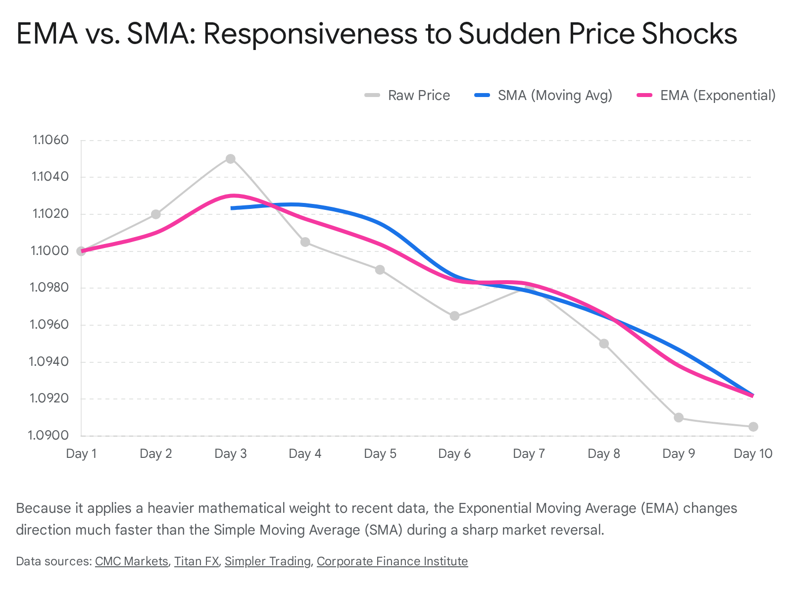
The defining characteristic of the SMA is that it applies equal weight to every single observation in the data set [15, 16, 17, 19]. The price from ten days ago exerts the exact same mathematical influence on the current SMA value as the price from yesterday [15, 17, 19]. This equal distribution of weight creates a highly stable, smooth line that is excellent for determining broad, long-term trends [15, 16, 18]. However, this stability comes at the cost of significant lag [10, 15]. When a market experiences a sudden, violent reversal, the SMA is notoriously slow to reflect the change, as the new data must fight against the equal weighting of older, obsolete data [15, 16, 17].
The Exponential Moving Average (EMA)
The Exponential Moving Average (EMA) was engineered specifically to solve the lagging deficiencies of the SMA [15, 17, 19]. Instead of treating all historical data equally, the EMA utilizes a complex weighting multiplier that places disproportionately higher significance on the most recent trading days [1, 15, 16, 17, 19].
Through an iterative formula, today's price affects the EMA more heavily than yesterday's, which in turn affects it more heavily than the day prior [15, 16]. This exponential decay of historical data points causes the EMA line to "hug" the current price action much more tightly [15, 17, 20]. Consequently, the EMA reacts with high velocity to sudden price shocks and momentum shifts, making it the preferred tool for active swing traders who need to capture short-term moves before they dissipate [1, 5, 8, 16, 17, 19].
Advanced and Niche Moving Averages
While the SMA and EMA dominate the landscape, quantitative analysts have developed other variations to balance the trade-off between smoothing and responsiveness [15, 30]. The Linear Weighted Moving Average (LWMA) forces a rigid, linear drop-off in weight rather than an exponential one [15, 44]. The Double Exponential Moving Average (DEMA) and Triple Exponential Moving Average (TEMA) apply multiple layers of exponential smoothing to virtually eliminate lag, though this extreme sensitivity makes them highly susceptible to false signals [30, 44]. Finally, the Triangular Moving Average (TMA) places the heaviest mathematical weight on the middle portion of the data series, creating a uniquely sluggish but incredibly smooth line that ignores almost all sudden volatility [68, 81].
| Indicator Type | Weighting Mechanism | Primary Characteristic | Optimal Swing Trading Application |
|---|---|---|---|
| Simple (SMA) | Equal weight to all data points. | High stability, slow reaction [15, 16, 17]. | Defining structural, long-term macroeconomic trends (e.g., 200-day) [15, 16]. |
| Exponential (EMA) | Front-loaded; exponential decay of old data. | High sensitivity, fast reaction [15, 16, 17]. | Timing short-term and intermediate swing entries (e.g., 20-day) [5, 6, 8]. |
| Linear Weighted (LWMA) | Linear decrease in weight toward older data. | Moderate sensitivity [15, 44]. | Custom short-term trend filtering [15]. |
| Triangular (TMA) | Heaviest weight placed on the middle data points. | Extreme smoothness, heavy lag [68, 81]. | Filtering out massive volatility spikes in highly chaotic markets [68, 81]. |
The Swing Trader's Timeframe Philosophy
In financial markets, technical indicators must be calibrated to the trader's specific holding period. Day traders and high-frequency scalpers operate on minute-by-minute charts, utilizing ultra-fast moving averages to capture microscopic fluctuations [9, 16, 33]. Conversely, deep-value investors may look at multi-year moving averages on monthly charts to assess generational macroeconomic shifts [54, 82].
Swing trading rests firmly in the middle. The objective of a swing trade is to capture a sustained "swing" in price momentum that lasts a minimum of one day and up to several weeks [4, 6]. Because of this hybrid holding period, swing traders require indicators that are responsive enough to signal a developing trend early, yet resilient enough to prevent the trader from being shaken out by a single day of random market noise [4, 7, 9].
Through decades of empirical trial and error, the swing trading community - and institutional finance at large - has gravitated toward three standard moving average lengths. These three lines function as a comprehensive system, layering fast momentum, intermediate filtering, and long-term bias [5, 6, 8, 9, 44].
The Pulse of Momentum: The 20-Period Average
The 20-period moving average (most frequently deployed as an EMA) represents approximately one month of trading data on a daily chart [5, 6, 7]. It serves as the primary gauge for aggressive, short-term momentum [6, 7, 8, 11].
When an asset's price rides consistently above the 20-day EMA, it signals that buyers are firmly in control of the immediate narrative [7, 11, 46]. Pullbacks to the 20-day EMA in a strong tape are often viewed as quick, high-probability entry points for short-term swing trades [6, 11]. However, because it is tethered so closely to recent price action, the 20-day average is highly susceptible to generating false signals when the market is choppy [7, 46]. A single volatile news event can easily push an asset below its 20-day line, only for the price to recover the very next day [12, 13, 14, 50].
The Intermediate Filter: The 50-Period Average
The 50-day moving average acts as the anchor for intermediate swing trading [5, 6, 8, 11, 45, 46]. Encompassing roughly ten weeks of historical data, it strikes a critical balance: it filters out the erratic noise that plagues the 20-day average, yet it still tracks the evolving trend far more accurately than longer-term metrics [7, 9].
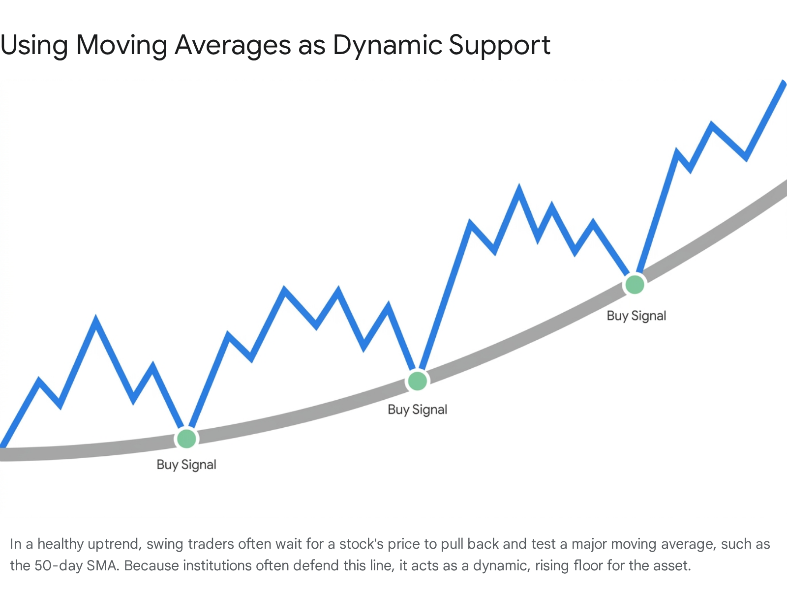
The 50-day SMA or EMA holds profound psychological and operational weight across global financial markets [11, 45, 46]. It is heavily monitored by institutional portfolio managers, mutual funds, and algorithmic trading systems [5, 11, 45, 46]. Because such vast amounts of capital are programmed to interact with this specific average, it frequently becomes a self-fulfilling prophecy [11, 46]. In a robust uptrend, institutional buyers often wait for an asset to pull back to its 50-day average before adding to their positions, creating a massive influx of demand exactly at that mathematical line [11, 46]. For a swing trader, the space between the 20-day and 50-day moving averages is often designated as a primary "buy zone" for entering a developing trend [8, 9].
The Macroeconomic Baseline: The 200-Period Average
The 200-day Simple Moving Average is the undisputed benchmark of long-term trend analysis, capturing roughly one calendar year of market behavior [2, 5, 6, 11, 45, 46]. It is widely considered the ultimate dividing line between structural bull markets and structural bear markets [11, 45, 46, 48].
Swing traders generally do not use the 200-day average for timing precise daily entries, as its extreme lag renders it practically useless for short-term maneuvers [5, 6, 10, 16]. Instead, it serves as a supreme context filter [5, 8, 9, 10]. A fundamental rule of systematic swing trading is to align short-term trades with the primary macroeconomic trend [8, 9]. If an asset is trading below its declining 200-day SMA, the macro environment is bearish; taking "long" (buy) setups in this environment is statistically dangerous, as the trader is fighting the dominant tide of capital [6, 11, 48]. Conversely, executing bullish swing trades when the asset is firmly above a rising 200-day SMA significantly increases the probability of success [5, 8, 11, 48].
Extracting Actionable Signals: How Traders Apply the Averages
Moving averages do not possess inherent predictive qualities; they merely visualize a smoothing formula [15, 25]. However, the ways in which current price interacts with these smoothed lines can reveal critical insights regarding supply, demand, and shifts in market psychology [1, 3, 5, 9]. Swing traders extract value through three primary methodologies: trend slope analysis, dynamic support and resistance, and moving average crossovers.
Trend Slope and Price Proximity
The most fundamental application of a moving average is to observe its trajectory [2, 10, 11, 46]. If a 50-day moving average is sloping upward from the bottom left of the chart to the top right, the intermediate trend is definitively positive [2, 7]. Furthermore, the proximity of the raw price to the moving average indicates the strength of the trend. If the price is stretching far above an ascending moving average, the asset may be temporarily overbought and due for a pullback [5, 9, 23].
If the moving averages flatten into horizontal lines and begin entangling with the raw price, it signals that the market has lost its directional momentum and has entered a sideways consolidation phase [6, 11, 46]. During these flat periods, swing traders typically avoid trend-following strategies altogether, as the market lacks the necessary directional thrust to yield profitable swings [11, 46].
Dynamic Support and Resistance
In classical technical analysis, support and resistance are depicted as static horizontal lines drawn across historic price peaks and troughs [3, 29, 42]. These lines represent fixed price points where buyers or sellers historically congregated [3, 6].
Moving averages, conversely, function as dynamic levels of support and resistance that evolve alongside the price action [1, 3, 6, 9]. As an asset trends upward, traders who missed the initial breakout often refuse to chase the inflated price. Instead, they wait for a mean-reversion event - a temporary pullback where the price dips to meet the rising moving average [1, 4, 6, 9, 11]. When the price touches the 20-day or 50-day EMA, these waiting buyers execute their orders en masse, causing the price to bounce [1, 3, 6, 11]. The moving average thereby acts as a rising floor, or dynamic support [1, 3, 6].
In a downtrend, the inverse is true. Rallies toward a descending moving average are often met with heavy selling pressure from investors desperate to exit losing positions, turning the moving average into a descending ceiling, or dynamic resistance [1, 3, 9]. Swing traders build their entire risk-management frameworks around these zones, entering trades as the price approaches the dynamic support and placing protective stop-loss orders just below the moving average line to strictly limit potential losses [4, 6, 8, 46].
Crossover Trading Systems
A crossover strategy is a systematic methodology that plots two or more moving averages of differing lengths on the same chart [1, 2, 5, 8, 10, 18, 47, 48]. A mechanical trading signal is generated at the exact moment the lines intersect [1, 2, 8, 10, 18, 47].
The underlying thesis of a crossover is that when a fast, short-term average cuts through a slow, long-term average, it provides mathematical confirmation that recent momentum is overpowering historical inertia [5, 8, 10, 18, 48].
- The Golden Cross: This is widely considered the most famous technical signal in global finance [1, 5, 10, 11, 29, 36, 47]. A Golden Cross occurs when the 50-day moving average climbs above the 200-day moving average [1, 5, 10, 11, 29, 36, 47, 75]. It implies that intermediate momentum has firmly reversed a prior downtrend and that a sustained, macroeconomic bull market is likely underway [5, 10, 36, 47, 75].
- The Death Cross: The inverse of the Golden Cross, a Death Cross materializes when the 50-day moving average plummets below the 200-day average [8, 10, 25, 29, 36, 47, 75]. It is viewed as a dire warning that heavy distribution is occurring and a prolonged bear market is imminent [10, 25, 36, 75].
- Short-Term Swing Crosses: Because the 50/200 crossover is remarkably slow to develop - often triggering months after a bottom has been reached - swing traders deploy much faster combinations for weekly trading [8, 11]. Common pairings include the 9-day EMA crossing the 20-day EMA, or the 10-day SMA crossing the 30-day EMA [8, 48]. These rapid crossovers allow traders to enter and exit momentum swings with agility, though they produce significantly more false signals [8, 14, 48].
The Limitations of Lag: The Rearview Mirror Problem
While moving averages introduce a semblance of order to chaotic charts, they are burdened by profound mathematical limitations [10, 15, 25, 27, 49, 50, 51]. Treating them as infallible predictive algorithms is a psychological trap that consistently devastates amateur traders [25, 49, 50].
By sheer definition of their mathematical formulas, all moving averages are lagging indicators [10, 11, 15, 25, 26, 27, 28, 29, 30]. Unlike leading indicators - such as the Relative Strength Index (RSI) or Stochastic oscillators, which attempt to predict reversals before they happen by measuring overbought or oversold extremes - moving averages can only react to what has already been logged in the historical record [26, 27, 28, 30, 67].
They do not forecast future price movement; they merely confirm historical trends [25, 26, 27, 28, 29]. As one market analyst aptly summarized, utilizing a moving average to navigate financial markets is similar to "trying to drive your car by only looking in the rearview mirror" [25]. If a corporation unexpectedly announces bankruptcy or the central bank abruptly shifts interest rates, the raw price of the asset will instantly collapse [25, 49]. However, the 50-day and 200-day moving averages, burdened by months of prior high prices, will barely register a dip on the day of the crash [10, 15, 25, 27]. By the time the moving averages slowly bend downward to formally trigger a "sell" signal or a Death Cross, the catastrophic damage to the portfolio has already occurred [10, 11, 17, 25, 27].
The Sideways Market Trap and "Whipsawing"
The utility of moving averages is strictly confined to trending environments [10, 11, 12, 13, 29, 46]. When an asset is actively climbing or falling, moving averages brilliantly track the slope [10, 11, 12]. However, markets do not permanently trend. Assets spend vast amounts of time in consolidation phases, grinding sideways in choppy, directionless ranges as buyers and sellers fight to establish a new equilibrium [10, 11, 12, 13, 29].
In a sideways market, moving averages become a severe liability [6, 11, 12, 13, 46]. Because the price is oscillating up and down within a tight horizontal band, the moving averages flatten out and converge [11, 13, 46, 50]. The short-term average will rapidly cross above the long-term average, triggering a technical "buy" signal [13, 50]. A swing trader executes the purchase, only for the price to instantly reverse and plummet below the averages the following day, triggering a "sell" signal for a loss [12, 13, 25, 50].
This brutal cycle of buying late into false rallies and selling low into false drops is known as "whipsawing," and it is exceptionally destructive to trading capital [10, 11, 12, 13, 14, 16, 46]. The quantitative reality of whipsawing is stark: an extensive historical backtest of simple crossover systems on the S&P 500 spanning from 1960 to 2025 demonstrated that certain moving average configurations generated false, money-losing signals at an alarming rate of up to 76% [14]. When an asset transitions from a trend into a choppy range, the optimal application of moving averages is to ignore them entirely [11, 13, 46].
The Academic Consensus: Profitability vs. The Efficient Market
The widespread reliance on moving averages has fueled a long-standing, intense debate within financial academia [31, 32, 41, 42, 60, 62]. For much of the late 20th century, traditional economic theory was dominated by the Efficient Market Hypothesis (EMH), formalized by Eugene Fama in 1970 [41, 52, 61, 70, 73].
The "weak form" of the EMH posits that current asset prices instantly and perfectly reflect all historical pricing data and volume [41, 52, 70, 73]. Therefore, analyzing historical data patterns - which is the exact definition of technical analysis and moving average trading - cannot possibly yield an informational edge or generate excess market returns [41, 52, 70, 73]. Early academic reviews largely dismissed moving averages as unscientific "black magic" or an optical illusion that merely preyed on the human brain's desire to find order in chaos [41, 53, 62].
However, the advent of massive computational power in the 21st century allowed researchers to exhaustively backtest tens of thousands of moving average strategies against millions of data points across global markets [33, 41, 54, 72, 73]. This modern era of research has produced a highly nuanced consensus that challenges strict interpretations of the EMH while simultaneously sobering the expectations of amateur traders [32, 33, 41, 42, 60].
Performance Against "Buy and Hold"
When academic literature evaluates moving average strategies, the standard benchmark is always a passive "buy-and-hold" strategy (buying an index and doing nothing for decades) [35, 36, 37, 38, 55, 66, 74]. The overwhelming consensus of extensive historical backtesting is that active moving average crossover strategies rarely, if ever, outperform the pure, absolute returns of passively holding a major index [31, 35, 37, 38, 55, 66, 74, 78, 86].
A definitive study analyzing the S&P 500 Index over a 65-year period (from 1951 to 2016) found that strictly following a 200-day moving average strategy yielded an annualized return of 7.11% [58, 78]. Over the exact same timeframe, a passive buy-and-hold approach yielded 7.24% [58, 78]. Comprehensive tests involving 36 different moving average rules across the United States and the United Kingdom further corroborated this, concluding that not a single moving average combination bested the long-term returns of buying and holding the broad market [37].
The economic realities become even bleaker for moving average strategies when the inherent frictions of active trading are applied to the models [31, 34, 41, 77, 84]. Executing trades based on daily or weekly moving average crossovers requires constant buying and selling [84]. Each transaction incurs tangible costs: broker commissions, bid-ask spread slippage, and potential short-term capital gains taxes [43, 66, 77, 84].
A stringent simulation testing the popular 50/200 EMA crossover on the SPY and NVDA tickers using realistic execution costs (5 basis points of slippage and 2 basis points for commissions per trade) revealed that the strategy rapidly collapsed [77]. The constant friction of transaction costs, combined with the low win rates caused by whipsawing in sideways markets, entirely eroded the statistical edge of the crossover system [77, 84].
Inefficiencies in Emerging Markets and Firm Life Cycles
Interestingly, while moving averages struggle to beat the highly efficient, heavily capitalized markets of the United States and Western Europe, academic studies have identified anomalous profitability in emerging markets [36, 37, 43, 65, 70, 73, 86].
Extensive research into the BRICS nations (Brazil, Russia, India, China, and South Africa), as well as the Romanian and Malaysian stock exchanges, indicates that moving average crossover rules generated statistically significant excess returns compared to passive holding in those specific regions [36, 43, 64, 65, 70, 86, 87]. This phenomenon suggests that developing equity markets suffer from slower information dissemination, lower liquidity, and higher retail speculation [36, 37, 43, 65, 73]. Because it takes longer for fundamental information to be fully priced in, these markets generate smoother, longer-lasting trends that moving average algorithms can successfully exploit before the momentum exhausts itself [36, 37, 43, 65, 73].
Furthermore, researchers analyzing the Taiwanese market discovered a distinct "U-shape" in the profitability of moving average strategies based on a firm's specific life cycle [39, 40, 69]. Trend-following algorithms were highly profitable when trading young, highly volatile companies in their introduction phase, or struggling companies in their decline phase [39, 40, 69]. In both extremes, public information uncertainty is exceptionally high, leading to delayed market reactions and prolonged price trends [39, 40, 69]. However, when moving averages were applied to mature, stable "cash cow" companies, the strategy failed to generate any meaningful edge [39, 40, 69].
| Market Context | Moving Average Performance vs. Buy & Hold | Primary Academic Explanation |
|---|---|---|
| Developed Western Markets (e.g., S&P 500) | Underperforms or matches [37, 58, 66, 74, 78]. | High efficiency, rapid information pricing, heavy trading frictions erode edge [37, 77, 84]. |
| Emerging Markets (BRICS, Malaysia, Romania) | Outperforms historically [36, 43, 64, 65, 70, 86, 87]. | Delayed information processing creates longer, exploitable trends [36, 37, 43, 65]. |
| Early-Stage/Declining Companies | Outperforms [39, 40, 69]. | Information uncertainty leads to underreactions and sustained momentum swings [39, 40, 69]. |
| Mature/Stable "Blue Chip" Companies | Underperforms [39, 40, 69]. | High certainty and stability mean prices rapidly reflect intrinsic value, limiting trends [39, 40, 69]. |
The True Utility: Risk Mitigation and Drawdown Truncation
If moving average crossover strategies consistently fail to generate massive, market-beating returns in major indices, why do institutional investors, algorithmic hedge funds, and professional swing traders continue to utilize them? The answer lies in risk management and behavioral psychology [11, 28, 58, 68, 74, 78, 81, 82].
While moving averages drag slightly on absolute cumulative returns during raging bull markets, academic studies universally agree that they drastically reduce portfolio volatility and severe drawdowns [31, 58, 65, 68, 74, 78, 81, 82]. By utilizing a strict rule - such as liquidating all equity positions into cash the moment the S&P 500 crosses below its 200-day moving average - a systematic strategy effectively bypasses the most catastrophic elements of financial collapses [58, 74, 78].
In a secular bear market, such as the Dot-Com crash of 2000 or the Global Financial Crisis of 2008, a buy-and-hold investor suffered excruciating losses of over 50% of their portfolio's value. A trader strictly adhering to a 200-day moving average strategy experienced minor whipsaw losses at the onset of the crash, but spent the vast majority of the devastating bear market safely sidelined in cash [58, 74, 78]. Consequently, while the moving average strategy may slightly underperform in raw percentages over 60 years, it produces a significantly higher "Sharpe Ratio" (a metric measuring risk-adjusted return) because the investor is not subjected to ruinous volatility [58, 64, 67, 74, 78, 82].
For the modern swing trader, the moving average is less of a predictive weapon and more of a defensive shield [11, 28, 46]. It forces emotional human beings to adhere to a rigid, mathematical discipline [11, 45, 46, 74]. It objectively demands that a trader stop attempting to buy falling assets in a macro downtrend, and provides unambiguous, visible levels to place stop-loss orders [6, 11, 45, 46].
Bottom line
A moving average is a foundational statistical tool that cuts through the daily chaos of financial markets, allowing swing traders to objectively identify momentum, define the macro trend, and interact with dynamic support and resistance levels. While variations like the exponential moving average (EMA) offer faster reaction times, all moving averages are inherently lagging indicators that can inflict severe "whipsaw" losses during directionless, sideways markets. Ultimately, rigorous academic backtesting proves that moving average strategies rarely beat a simple buy-and-hold approach in raw returns, but they remain invaluable to professionals because they enforce strict trading discipline and drastically mitigate catastrophic risk during severe market collapses.