Non-Stationarity and Concept Drift in Quantitative Trading
Statistical Foundations of Market Non-Stationarity
In the discipline of quantitative finance, the assumption that historical market data distributions will persist into the future constitutes the primary vulnerability of algorithmic trading models. Financial markets are inherently non-stationary; their statistical properties - including means, variances, and cross-asset correlations - fluctuate continuously. These fluctuations are driven by macroeconomic developments, regulatory shifts, technological advancements, and the endogenous feedback loops generated by market participants. Time series analysis relies heavily on the concept of stationarity, which assumes the stability of statistical properties over time 1. When the underlying data-generating process evolves, models trained on historical data experience severe performance degradation, a phenomenon broadly categorized as model decay.
The proliferation of machine learning and deep reinforcement learning in quantitative strategies has amplified the complexity of diagnosing and mitigating this issue. While deep neural networks excel at extracting non-linear patterns from vast, high-dimensional datasets, their performance is acutely sensitive to distribution shifts. Consequently, quantitative researchers must isolate the exact mechanisms of model decay to engineer adaptive methodologies capable of identifying and responding to real-time regime shifts.
Distinctions Between Data Drift, Concept Drift, and Label Shift
Model decay is not a monolithic phenomenon. It is the observable outcome of varying types of distributional shifts within the input data or the functional relationships between inputs and outputs. In supervised financial machine learning, the training dataset is typically viewed as a set of samples from a joint distribution $P(X, Y)$, where $X$ represents the input features (e.g., limit order book depth, technical indicators, macroeconomic variables) and $Y$ represents the target variable (e.g., forward returns, volatility). The degradation of the predictive conditional probability model $P(Y|X)$ originates from distinct distributional shifts 234.
| Shift Classification | Statistical Definition | Financial Market Manifestation | Required Adaptive Response |
|---|---|---|---|
| Data Drift (Covariate Shift) | $P(X)$ changes, but $P(Y|X)$ remains constant. | A new regulatory framework permanently alters the average daily volume of an asset. The input distribution of volume changes, though the relationship between volume spikes and price impact holds. | Feature re-scaling, continuous normalization, or updating the input training distribution without altering the core model architecture. |
| Concept Drift | $P(Y|X)$ changes, but $P(X)$ remains constant. | The historical relationship where high inflation predicts higher equity returns breaks down, and high inflation begins to predict severe equity drawdowns. The inputs remain within normal bounds, but the target relationship is inverted. | Continuous retraining, online learning algorithms, adaptive windowing, or Markov regime-switching models. |
| Label Shift (Prior Shift) | $P(Y)$ changes, but $P(X|Y)$ remains constant. | A prolonged macroeconomic expansion significantly increases the overall baseline probability of positive daily returns across the market, independent of specific asset technical features. | Adjusting class priors or utilizing re-weighting techniques to account for the new baseline market probability. |
Concept drift is generally considered the most disruptive factor in algorithmic trading. When concept drift occurs, the model continues to make predictions with high statistical confidence, entirely unaware that the underlying logic it learned during the training phase is no longer valid in the live market 56. When historical correlations invert or volatility regimes abruptly transition, the exact same inputs reliably produce vastly different outputs, rendering static models highly unprofitable.
The Mechanics of Trading Model Decay
To systematically address the degradation of trading models, analysts must distinguish between genuine structural breaks in the market and the inevitable failure of poorly constructed algorithms. The quantification of backtest decay is transitioning from a descriptive diagnostic into a formal inferential standard in financial machine learning.
Backtest Overfitting Versus Genuine Drift
A persistent challenge in quantitative research is differentiating actual concept drift from backtest overfitting. Strategies developed to perform exceptionally well on a specific historical sample often monetize random historical noise rather than genuine market inefficiencies. When these strategies are deployed out-of-sample and subsequently fail, the failure is frequently misattributed to a sudden market regime shift, when in reality, the model never possessed true predictive power 789.
Standard statistical techniques, such as standard hold-out validation, are considered insufficient for financial time series due to the multiple testing problem. When analysts iteratively test varying parameter combinations and select the best-performing model, they induce severe selection bias, mathematically inflating the expected maximum performance 84.
To quantify and control for this selection-induced backtest inflation, advanced falsification frameworks utilize the Deflated Sharpe Ratio (DSR). The DSR adjusts the standard Sharpe ratio by accounting for the variance of the tested Sharpe ratios across all trials, the non-normality of the strategy's returns, and the effective multiplicity of the research process 4115. Furthermore, techniques such as Combinatorial Purged Cross-Validation (CPCV) are employed to prevent data leakage across temporal boundaries. CPCV involves purging and embargoing data adjacent to the test set, ensuring that any subsequent out-of-sample decay can be confidently attributed to actual concept drift rather than the unwinding of an overfit parameter set 86.
The Hyperbolic Decay of Factor Alpha
Model decay is also driven by endogenous market factors, primarily the competitive crowding of trading strategies. As specific quantitative signals - or alpha factors - are discovered and capitalized upon by multiple market participants, the aggregate market impact of their collective execution erodes the profitability of the signal.
Recent game-theoretic equilibrium modeling suggests that factor alpha decay follows a specific hyperbolic functional form, expressed as $\alpha(t) = K / (1 + \lambda t)$, rather than a standard linear or exponential decline 14. This hyperbolic decay is particularly pronounced in "mechanical" factors, such as systematic momentum, where the signal rules (e.g., buying recent winners) are unambiguous and easily replicated by competing funds. While exponential decay assumes a constant half-life, hyperbolic decay indicates that alpha degrades more slowly initially but leaves a heavier, persistent tail of low-level profitability as marginal capital eventually exits the crowded trade 14. Out-of-sample testing from 2001 to 2024 demonstrates that crowded reversal factors show significantly higher crash probabilities, whereas the hyperbolic model successfully predicts the longer-term stabilization of momentum factors 14.
Historical Regime Shifts and Model Failures
The theoretical vulnerabilities of static models manifest dramatically during historical regime shifts. A market regime is defined not merely by a volatility state, but by a cohesive combination of liquidity conditions, correlation structures, policy sensitivities, and dominant behavioral feedback loops 15.
The Inflation Pivot and Quantitative Performance Bleed
The macroeconomic environment spanning from the post-2008 Global Financial Crisis to late 2021 was broadly characterized by low inflation, accommodative central bank monetary policy, and abundant liquidity. This era, often dubbed the "Great Moderation," fostered highly stable inter-asset correlations and predictably low volatility 16. However, the global inflation surge of 2022 prompted aggressive monetary tightening, effectively terminating this regime.
This transition resulted in severe decorrelation events between traditionally inversely correlated assets. Under normal conditions, the S&P 500 and the VIX maintain a strong negative correlation. However, structural breaks led to periods where equities and volatility decoupled, undermining the foundational assumptions of many volatility-targeting and risk-parity models 1718. The result was not a singular market crash, but rather a prolonged "slow bleed" in the performance of many systematic quantitative hedge funds extending through 2023 and into 2025. Funds operating models overfit to the low-inflation, mean-reverting regime repeatedly executed historical playbooks in an environment that had transitioned to persistent momentum, accumulating steady losses as their algorithms fell out of sync with new market realities 1920.
The underlying mechanics of these shifts follow a specific structural progression. They begin with an initial quiet phase where market breadth narrows and liquidity becomes selective. This is followed by a compression phase where correlations creep higher and small shocks generate outsized reactions, culminating in the observable regime break indicated by sustained, elevated volatility 1521.
Options Markets and Second-Order Risks
The perils of concept drift are magnified in strategies involving complex derivatives and non-linear payoffs. In options markets, strategies such as gamma scalping rely heavily on the empirical assumption that implied volatility will persistently overestimate realized volatility 22. The delta-hedged long-gamma strategy systematically loses money on average under standard conditions, meaning funds often sell options to capture the volatility risk premium 22. During regime shifts, the rapid expansion of realized variance can eviscerate these short-volatility models.
The collapse of the Allianz Structured Alpha fund serves as a prominent institutional case study in model manipulation and structural failure. The fund utilized a strategy that targeted alpha by collecting premium through selling out-of-the-money put and call spreads on the S&P 500, theoretically relying on modeled downside protection positions 22. When the COVID-19 pandemic induced an unprecedented volatility regime shift in March 2020 - with the VIX spiking from near 15 to an intraday high of 82.69 - the strategy's risk models decayed instantly. Post-collapse investigations revealed that the portfolio managers had systematically altered Greek reports, manually reducing downside gamma exposure inputs to hide the true risk of the regime shift 1622. The speed of the transition outpaced the static model's ability to adjust hedges naturally, exposing the severe vulnerabilities of static risk modeling during a sudden structural break.
Emerging Markets and Commodity Dislocation
Commodity markets and emerging market (EM) equities are highly susceptible to rapid regime shifts due to geopolitical shocks, supply-chain sensitivities, and currency fluctuations. Between 2022 and 2024, energy and agricultural commodities experienced severe price dislocations driven by the Russia-Ukraine conflict, global inflation, and extreme weather anomalies 7. Research has demonstrated that during these periods, the traditional risk-return profiles of EM portfolios deteriorated rapidly, increasing their correlation with developed markets and eliminating expected diversification benefits 89.
In response, quantitative researchers have utilized statistical modeling to identify distinct regimes. Foreign exchange models have integrated four-state regime-switching frameworks to define market conditions based on the magnitude of deviation from long-term trends, allowing optimal hedge ratios to adapt to the fat-tail properties of highly volatile currencies like the Turkish Lira and Japanese Yen 1011. By recognizing that traditional assumptions fail during geopolitical shocks, adaptive asset allocation systems can outperform static buy-and-hold strategies by adjusting exposure dynamically as the probability of a high-volatility state increases 1230.
Regime Detection and Statistical Modeling
Identifying the exact moment a regime transitions is critical for deploying adaptive trading strategies. Volatility serves as a primary signal; however, raw volatility must be statistically parsed to detect true structural breaks rather than transient noise.
Markov-Switching and Autoregressive Models
To circumvent the limitations of fixed-parameter models, researchers employ Markov-switching autoregressive models and Hidden Markov Models (HMM). These models do not assume a single data-generating process; instead, they assume the market oscillates between multiple hidden states (e.g., a low-volatility growth state and a high-volatility contraction state) 3013.
HMMs rely on state graphs defined by initial state probabilities, state transition probabilities, and observation emission probabilities. Algorithms such as Baum-Welch or Viterbi are used to estimate the underlying hidden states given observed price data 13. Empirical testing on the S&P 500 demonstrates that HMMs successfully identify historical crash periods, including the 2008 financial crisis and the 2020 pandemic shock, allowing associated investment strategies to pivot defensively and outperform static baselines 13. Similarly, Generalized Autoregressive Conditional Heteroskedasticity (GARCH) models are utilized to forecast the persistence of volatility clusters, adapting to the phenomenon where large price swings are typically followed by subsequent large swings 168.
Causal Discovery in Non-Stationary Environments
Standard predictive models often capture spurious correlations that collapse during regime shifts. Causal discovery algorithms attempt to map the actual structural dependencies between financial variables. However, traditional causal discovery assumes data stationarity. When analyzing time-series data with distributional shifts, standard approaches yield false causal relations. Recent frameworks have been developed specifically to handle non-stationary time-series data, detecting both lagged and contemporaneous causalities without relying on the assumption that the non-stationarity is consistent across time 32. This allows models to identify robust signals that persist regardless of the broader market regime.
Adaptive Forecasting Methods in Time Series Analysis
To combat non-stationarity, quantitative modeling is shifting toward highly adaptive, dynamic frameworks. Traditional statistical methods like standard ARIMA maintain fixed parameters after initial training, leaving them vulnerable to structural breaks. Modern solutions focus on dynamic windowing and deep learning architectures.
The Nonstationarity-Complexity Tradeoff
Adaptive strategies frequently employ a rolling-window methodology, periodically retraining the model on the most recent slice of historical data to capture the current regime. However, this introduces a fundamental nonstationarity-complexity tradeoff in financial machine learning. As model complexity increases, misspecification error decreases, allowing the model to capture intricate market dynamics. However, complex models require much larger training windows to achieve statistical significance and avoid overfitting. Expanding the training window inadvertently increases the model's exposure to non-stationarity risk, as market regimes are highly likely to shift over an extended timeline, thereby punishing the obsolete complexity of the model 3334.
To resolve this tension, researchers have developed online, data-driven mechanisms to dynamically manage window size. Algorithms like the Adaptive Tournament Of Model/Window Selection (ATOMS) evaluate combinations of models and window lengths via adaptive pairwise validation. By evaluating candidates on non-stationary validation data, the system statistically expands the window during stable periods to reduce variance, and drastically shrinks the window when distributional breaks are detected to minimize bias 3334. Applied to industry portfolio returns, these adaptive methods consistently outperform standard rolling-window benchmarks, particularly during designated recessionary periods 34.
Deep Learning Architectures and Sequence Representation
The application of deep learning to financial time series introduces significant scalability and flexibility. However, empirical benchmarking reveals nuances in architecture selection when dealing with non-stationary data.
| Architecture Type | Examples | Performance Characteristics on Financial Data |
|---|---|---|
| Linear Models | DLinear, NLinear | Decompose inputs into trend and seasonal components, or operate on normalized inputs. Highly stable and act as strong baselines, often outperforming overly complex neural networks by avoiding severe overfitting to noise 3514. |
| Recurrent Networks | LSTM, GRU | Capture temporal dependencies effectively. Enhanced variants (e.g., xLSTM) demonstrate strong balance between performance and stability, improving robustness to trading frictions and intertemporal consistency across market regimes 3537. |
| Transformer Models | PatchTST | Utilize self-attention mechanisms. While successful in other domains, pure patching approaches can exhibit high sensitivity to specific temporal years in finance. They require augmentation with stronger sequence modeling (e.g., LPatchTST) to achieve stable temporal state encoding 3514. |
Deep networks frequently encounter challenges like overfitting, where models excel on training data but struggle to generalize to unseen, shifted distributions 91516. To extract stationary features from non-stationary price data without succumbing to this overfitting, researchers are increasingly operating in the frequency domain.
Methods such as Variational Mode Decomposition (VMD) break down non-stationary financial time series into smoother, more predictable subcomponents before feeding them into deep learning predictors like LSTMs, significantly improving model adaptability 17. More advanced architectures, such as the Deep Frequency Derivative Learning framework (DERITS), utilize Frequency Derivative Transformations to analyze the entire frequency spectrum, adjusting the distribution to acquire stationary representations without the information loss associated with simple mean-standardization 41.
Similarly, the Dual-branch Temporal and Frequency (DTAF) framework addresses non-stationarity across both domains simultaneously. It isolates and suppresses temporal non-stationary patterns using a Mixture of Experts (MoE) filter while tracking spectral shifts through frequency differencing, generating highly robust forecasts under dynamic conditions 18.
Another sophisticated hybrid approach is the Non-Stationary Transformer with Deep Reinforcement Learning (NSTD). This model actively mitigates data heterogeneity by concatenating macroeconomic indicators (GDP, CPI), sentiment-analyzed news streams using VADER scoring, and historical price data 19. It utilizes a specialized Transformer encoder equipped with temporal scaling and shifting factors - a "tau_learner" and "delta_learner" - to continuously recalibrate self-attention weights based on current non-stationary market conditions 19.
Deep Reinforcement Learning for Adaptive Execution
While supervised deep learning is largely limited to forecasting price trajectories, Deep Reinforcement Learning (DRL) extends the capability of AI into the realm of sequential decision-making. By formulating trading as a Partially Observable Markov Decision Process (POMDP), an RL agent interacts continuously with the market environment, updating its policy network through trial and error to maximize a cumulative reward function, typically structured around risk-adjusted returns net of transaction costs 202122.
Policy Optimization and Meta-Learning Architectures
State-of-the-art DRL implementations for algorithmic trading utilize model-free actor-critic architectures, including Proximal Policy Optimization (PPO), Advantage Actor-Critic (A2C), Soft Actor-Critic (SAC), and the Deep Deterministic Policy Gradient (DDPG). In architectures like DDPG, the actor network maps high-dimensional state representations - such as limit order book depth, rolling volatility, and remaining inventory - to continuous action spaces, which represent portfolio allocation weights or execution slicing sizes. Simultaneously, the critic network evaluates the expected value of those actions 194748.
Because standard RL agents trained on static historical environments assume fixed transition probabilities, they suffer catastrophic failure when live market dynamics drift. To counter this, modern systems integrate meta-learning and continuous adaptation paradigms. Instead of relying on a single monolithic policy, adaptive frameworks deploy ensembles of specialized sub-agents guided by a meta-controller. This hierarchical architecture allows the overarching system to rapidly swap to a mean-reversion policy, a momentum policy, or a defensive holding policy when distribution shifts are detected, maintaining profitability across differing macroeconomic regimes without requiring full offline retraining cycles 1948.
Execution Realism: Market Impact, Latency, and Transaction Costs
A critical flaw in early algorithmic trading research was the assumption of frictionless markets. When open-source DRL environments assume zero transaction costs, limitless liquidity, or fixed flat fees, agents inevitably learn pathological behaviors. They execute high-frequency, high-turnover strategies that appear highly profitable in theoretical backtests but incur ruinous slippage in live deployment due to market impact 4950. In reality, the execution of large orders shifts the limit order book against the trader, creating a fundamental trade-off between minimizing market impact through slow execution and managing price risk due to time delay 51.
Recent advancements address this discrepancy by integrating non-stationary limit order book dynamics and non-linear market impact models directly into the agent's training environment. For instance, the MACE (Market-Adjusted Cost Execution) environment utilizes the Almgren-Chriss framework and the empirical square-root impact law to penalize aggressive execution mathematically 5052.
When tested in these rigorous environments, the relative rankings of algorithms change drastically.
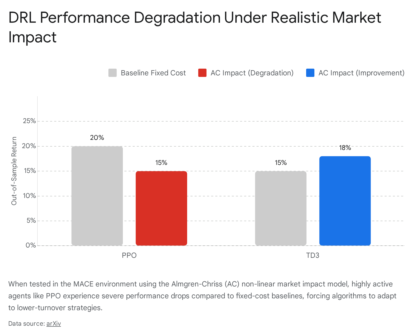
Under negligible fee assumptions, an unoptimized agent might execute trades resulting in a 19% daily turnover, generating massive theoretical returns but virtually guaranteeing systemic failure in production. However, when hyperparameter optimization is applied alongside the Almgren-Chriss cost penalty, the DRL agent organically learns to throttle its participation rate, dropping turnover to below 1% and executing passive limit-order schedules that drastically reduce execution decay 5052.
Furthermore, network latency - measured in milliseconds or microseconds - compounds this physical decay. High-frequency signals observed by an agent often dissipate before the resulting orders can cross the network and execute against the exchange matching engine 2354. Algorithms that operate with structural latency disadvantages are forced to cross the bid-ask spread aggressively, paying the liquidity premium. Adaptive reinforcement learning systems must therefore internalize not only the statistical drift of the asset price but the deterministic friction of the market microstructure itself 492456.
Conclusion
The persistence of model decay in quantitative trading underscores the severe limitations of static assumptions in a dynamic financial ecosystem. As market structures evolve through macroeconomic pivots, regulatory interventions, and the collective adaptation of algorithmic participants, historical patterns are continuously rewritten.
The essential distinction between temporary data drift and permanent concept drift requires rigorous falsification frameworks - such as Combinatorial Purged Cross-Validation and the Deflated Sharpe Ratio - to prevent researchers from conflating structural market breaks with the inevitable failure of overfit models. Moving forward, the resilience of systematic trading relies fundamentally on adaptive methodologies. These range from tournament-based rolling window selection and frequency-domain neural network transformations to continuous meta-learning in reinforcement agents. By embedding real-world frictions such as non-linear market impact and latency directly into the training phase, quantitative models can transition from brittle historical curve-fitting to robust, self-updating systems capable of navigating an inherently non-stationary world.