Impact of Market Regimes on Swing Trading Strategies
Financial markets are inherently non-stationary, meaning the underlying statistical distributions of asset returns continuously shift over time. For quantitative and discretionary swing trading strategies - which typically seek to capture multi-day to multi-week price movements - this non-stationarity poses a severe systemic challenge. A strategy optimized for a specific market environment will inevitably decay when that macroeconomic or microstructural environment transitions. This phenomenon, frequently misdiagnosed by market participants as standard alpha decay or flawed strategy logic, is more accurately defined as regime mismatch 12.
Extensive quantitative research, including multi-decade backtests across equity, commodity, and fixed-income indices, demonstrates that the success of swing strategies depends entirely on accurately identifying and adapting to the prevailing market regime 21. When traditional momentum or mean-reversion strategies are applied blindly across a 25-year dataset partitioned into distinct market regimes, the variance in risk-adjusted performance - measured by the Sharpe ratio - fluctuates by as much as 60% based solely on the active regime layer 2. Consequently, modern systematic trading has shifted away from rigid, static indicator-based execution and toward adaptive, regime-aware asset allocation, where the performance of technical indicators, the efficacy of stop-loss mechanisms, and the persistence of cross-asset correlations are continuously re-evaluated against probabilistic regime models.
Statistical Detection of Market Regimes
The classification of market regimes has evolved from heuristic technical definitions (such as moving average crossovers) to rigorous unsupervised machine learning and econometric models. These advanced frameworks analyze historical price action, volatility metrics, and cross-asset correlations to probabilistically determine the current market state without relying on biased ex-ante labels.
Hidden Markov Models and Regime Switching
The Markov Regime Switching (MRS) framework, initially popularized in econometrics, models financial time series by assuming that the observed data is generated by a process that transitions between multiple unobserved (latent) states 4. Each state, or regime, is mathematically characterized by its own set of parameters, typically the mean return and variance. This allows the model to partition historical data into distinct phases, such as low-volatility bull markets and high-volatility bear markets.
Standard Hidden Markov Models (HMM) utilize fixed transition probabilities and assume that the duration of a regime follows a geometric distribution. However, empirical financial data often contradicts this assumption, as market volatility regimes exhibit characteristic timescales that are not memoryless. To address this limitation, quantitative researchers employ Hidden Semi-Markov Models (HSMM), which explicitly model regime durations through non-geometric distributions, better capturing the prolonged persistence of structural bull markets and the sharp, short-lived nature of market crashes 2. Furthermore, score-driven models with time-varying transition probabilities (HMM-GAS) have been developed, where the likelihood of transitioning between states evolves dynamically based on the scaled score of the predictive likelihood, allowing the model to adapt to new observation data instantly without ex-ante specification of explanatory variables 2.
In comprehensive empirical testing, such as a 1,200 Monte Carlo simulation study conducted on daily S&P 500 returns spanning from 2003 to 2020, Markov models consistently demonstrate the profound structural inertia of stable markets 42. The transition probabilities extracted from these models reveal that the likelihood of the market remaining in a low-volatility regime, once established, is approximately 97.75% 4. Conversely, the probability of spontaneously transitioning from a low-volatility state to a high-volatility crisis state is notably low, measured at roughly 4.53% 4. This indicates that low-volatility conditions act as the default market state, while high-volatility periods are infrequent, highly disruptive shocks. Similar applications of Hidden Markov Models across 24 European stock indices over a 15-year period confirm this remarkable persistence of states, demonstrating that regime-switching coordination across global markets offers distinct risk-return tradeoffs that can be exploited for portfolio management 3.
| Regime Transition Path | Estimated Probability | Market Implication for Swing Strategies |
|---|---|---|
| Low Volatility → Low Volatility | 97.75% | High structural inertia; mean-reversion and premium collection strategies exhibit high win rates. |
| Low Volatility → High Volatility | 4.53% | Rare but severe systemic shocks; static stop-losses are vulnerable to overnight gap risk. |
| High Volatility → High Volatility | Variable (Regime Dependent) | Clustered volatility; trend-following strategies can capture extended momentum during sustained crises. |
| High Volatility → Low Volatility | Variable (Regime Dependent) | Market stabilization; transition back to equilibrium, favoring a return to mean-reversion tactics. |
Gaussian Mixture Models and Factor Lenses
While Markov models excel at modeling sequential time-series transitions, Gaussian Mixture Models (GMM) are frequently utilized to cluster multivariate financial data into discrete environments based on joint distributions. As an unsupervised machine learning method, a GMM uses multiple Gaussian distributions to model different segments of a dataset, with each distribution possessing unique means, volatilities, and correlation structures 4. This approach is particularly effective for financial assets, as it accurately captures both the central tendencies and the heavy tails (skewness) inherent in asset return distributions.
A prominent quantitative framework developed by Two Sigma applies a 17-dimensional GMM to model the joint distribution of various macro and style factors within the U.S. equities market 4. This algorithm identifies four distinct clusters representing core market conditions. The "Steady State" cluster represents healthy market periods where equity, credit, and style factors perform well with low volatility. The "Crisis" cluster is characterized by extremely poor performance in macro factors, negative mean returns for global equities, and positive returns for safe-haven factors like trend-following and low-risk styles 4. The "Inflation" cluster exhibits double-digit mean returns for local inflation factors while equities and interest rates underperform 4. Finally, the "Walking on Ice" regime identifies fragile market conditions or asset bubbles, where equity markets generate positive returns but exhibit significantly higher volatility than their long-term averages 4.
Another machine learning approach utilized by State Street Global Advisors employs a 4-state t-distributed mixture model integrated with Generalized AutoRegressive Conditional Heteroskedasticity (GARCH) 5. Analyzing 23 performance and uncertainty datasets from 1995 to 2024, the model classifies regimes into Robust Expansion, Emerging Expansion, Cautious Decline, and Market Turmoil 5. The Emerging Expansion regime, representing 42% of observations, is the most prevalent and acts as a transitional phase where risk assets begin exhibiting stronger returns alongside higher volatility 5. Because mixture models evaluate each period independently, they provide a point-in-time probability assessment of the current regime layer, functioning as a critical input for dynamic asset allocation.
Distance-Based Vector Matching
An alternative to strict parametric clustering is empirical distance matching. Rather than defining economic regimes via preset, rigid thresholds (such as defining inflation strictly as CPI > 4%), quantitative researchers calculate the Euclidean distance between current macroeconomic state variables and historical periods 67. A methodology developed by researchers at Man Group utilizes financial variables that embed macroeconomic information - including the S&P 500 index, yield curve slope, crude oil prices, copper prices, U.S. Treasury bill yields, equity market volatility, and stock-bond correlations 67.
These variables are transformed into annual changes and normalized using rolling z-scores to prevent look-ahead bias 6. The algorithm measures the multidimensional distance between the current month and every historical month in the dataset. Historical dates with the smallest aggregate distances are classified as "similar regimes," while those with the largest distances are classified as "anti-regimes" 67. This flexible, non-parametric approach systematically bypasses the limitations of traditional regime detection, allowing systematic swing models to position long or short equity factors based strictly on the actual forward returns observed in historically analogous environments 6. Portfolios constructed using this distance-matching technique have demonstrated statistically significant alpha generation across major market dislocations, including the 2008 Global Financial Crisis and the 2022 inflationary surge 7.
Technical Indicator Decay in Trending vs Range-Bound Environments
The core architecture of retail and institutional swing trading historically relies on technical indicators derived from price and volume data. However, empirical backtesting across multiple decades unequivocally demonstrates that the mathematical logic of these indicators decays rapidly when applied to an incompatible market regime 111. A strategy optimized for a directional trend will inevitably erode capital during periods of sideways consolidation.
Momentum and Mean-Reversion Divergence
Technical indicators are mathematically constructed to measure specific phenomena - either directional momentum or mean-reverting oscillation. Trend-following indicators, such as Exponential Moving Averages (EMAs) and the Moving Average Convergence Divergence (MACD), excel during periods of sustained directional movement. In trending regimes, price series exhibit positive autocorrelation, allowing these tools to capture extended multi-week swings and filter out minor retracements 128.
However, financial markets spend a significant portion of their time - frequently estimated at up to 70% - in non-trending, range-bound phases 9. During these consolidation periods, volatility compresses, moving averages flatten, and prices oscillate repeatedly between established horizontal support and resistance levels 915. In this specific regime, trend-following indicators suffer extreme mathematical decay. The MACD, for instance, consistently generates false zero-line crossovers, triggering erroneous entry signals that result in immediate whipsaw losses as the price reverses off the range boundary 15.
Conversely, bounded momentum oscillators like the Relative Strength Index (RSI) and the Stochastic Oscillator thrive in sideways consolidation 910. Unlike in trending markets where a strong directional move can keep an oscillator embedded in an "overbought" or "oversold" extreme zone for extended periods - generating premature and dangerous counter-trend signals - range-bound conditions allow these tools to reliably signal mean reversion 915.
A comparative quantitative study analyzing the efficacy of the RSI versus the MACD on the LQ45 index from August 2023 to July 2024 highlights this divergence perfectly. The empirical results demonstrated that the RSI achieved an exceptional accuracy level of 97% (31 successful signals out of 32) in identifying actionable reversals during the specific market conditions analyzed, whereas the MACD's accuracy dropped to 52% (86 successful signals out of 166) due to an abundance of false trend signals 1210. To synthesize these conflicting properties, sophisticated swing models dynamically adjust indicator parameters based on real-time volatility metrics. For example, a composite strategy might adjust the RSI overbought/oversold thresholds from the standard 30/70 to a tighter 25/75 strictly when historical volatility (HVIX) exceeds 20%, thereby buffering against false signals during transitions from range-bound to trending regimes 8.
Geopolitical Shocks and High-Frequency Noise
Indicator decay is severely accelerated during periods of exogenous market stress and high-frequency volatility. High-frequency trading (HFT) environments are dominated by market noise and microstructural fragmentation, rendering traditional price-based technical indicators highly susceptible to false signals 11.
Furthermore, during systemic geopolitical disruptions, the fundamental mechanics of technical analysis break down. A study analyzing the behavior of technical indicators during the onset of the Covid-19 pandemic revealed a marked deterioration in signal quality 12. Moving averages (such as the 50-day Simple Moving Average and 20-day Exponential Moving Average) showed sharply reduced amplitude and tighter values, failing to track the erratic and non-linear price movements. The MACD lost its consistency and responsiveness, while the RSI exhibited massive dispersion and instability, remaining elevated in extreme zones and suggesting constant market overreaction 12. The statistical effect of heightened volatility on these indicators is strictly negative; regression analysis confirms that each one-unit increase in volatility drastically reduces the reliability of trend-following metrics, necessitating the suspension of automated indicator-based swing execution during crisis regimes 12.
This structural fragility has forced modern quantitative funds to abandon static indicator combinations. Feature importance analyses conducted on Random Forest Regression models applied to minute-level stock data reveal that primary, raw price-based features and order flow consistently outperform derived technical indicators like Bollinger Bands and the Commodity Channel Index (CCI) in predictive accuracy 1113. While indicator-augmented machine learning models occasionally show improved risk-adjusted metrics in-sample, they struggle profoundly with out-of-sample generalization, proving that the inefficiencies identified by classical technical analysis are highly transient and lack persistence across shifting market regimes 1113.
| Indicator Classification | Optimal Market Regime | Mathematical Failure Condition |
|---|---|---|
| Moving Averages (SMA, EMA) | Trending (Positive Autocorrelation) | Range-Bound: Flattening slopes trigger continuous false crossovers. |
| Momentum Oscillators (RSI, Stochastic) | Range-Bound (Mean Reverting) | Strong Trend: Becomes embedded in extreme zones, prompting premature exits. |
| Volatility Bands (Bollinger, Keltner) | Volatility Expansion / Breakouts | Low Volatility: Bands compress tightly, failing to indicate directional bias. |
| Macro/Trend Systems (MACD, Parabolic SAR) | Structural Bull/Bear Markets | High-Frequency Noise: Lags significantly behind erratic, non-linear price shocks. |
Efficacy of Stop-Loss Mechanisms Across Regimes
The implementation of stop-loss rules is a foundational risk management principle in both discretionary and systematic swing trading. However, rigorous mathematical evaluation proves that the value added by stop-loss policies is not absolute; it is heavily dependent on the underlying statistical properties of the active market regime.
In classical financial theory, if asset prices are assumed to follow a standard Geometric Brownian Motion (GBM) - implying that returns are normally distributed and strictly independent (a random walk) - the optimal investment strategy is buy-and-hold 14. Under strict random walk conditions, any path-dependent strategy like a stop-loss rule merely diminishes expected earnings through accumulated transaction costs and premature liquidations. In this theoretical environment, a stop-loss acts essentially as a continuous insurance premium that degrades portfolio efficiency 14.
However, empirical financial markets do not operate as perfect random walks; they exhibit fractional Brownian motion (fBM), meaning that price series contain long-range dependence, structural autocorrelation, and fractal characteristics 2115. The true efficacy of a stop-loss is dictated by the Hurst parameter (H) of the asset's return distribution, alongside its expected drift and volatility 21.
When a market operates in a trending regime characterized by positive return autocorrelation (where the Hurst parameter is greater than 0.5), stop-loss rules substantially improve risk-adjusted returns 2116. In this environment, a stop-loss effectively truncates the left tail of the return distribution - limiting deep drawdowns and protecting capital - while allowing the right tail (the profitable trend) to persist 1516. Empirical analyses of commodity factor trading strategies reveal that trailing-stop strategies with dynamic thresholds perform exceptionally well in trending conditions, achieving an average Sharpe ratio of 1.28, compared to a Sharpe ratio of 0.92 for fixed-stop strategies, and significantly outperforming unmanaged buy-and-hold factors 21.
Conversely, in mean-reverting or range-bound regimes characterized by negative return autocorrelation (where the Hurst parameter is less than 0.5), the application of tight stop-losses becomes mathematically detrimental to the swing trader. Because price deviations in a sideways market are statistically likely to revert to the mean, premature liquidation triggered by a stop-loss forces the trader to lock in a realized loss just prior to the inevitable statistical rebound 21. In these choppy environments, stop-loss rules actively reduce absolute expected returns 21.
Furthermore, the mechanics of overnight gaps and flash crashes heavily impact stop-loss execution. Quantitative models that explicitly incorporate acute momentary price drops and overnight jump dynamics show that while stop-loss rules improve absolute expected returns in falling markets, the slippage incurred during a flash crash can severely erode the theoretical performance gains of the risk-management system 16. Consequently, systematic swing models must dynamically widen stop-loss distances during volatile, mean-reverting regimes to prevent high-frequency stop-outs, or suspend trading entirely until positive autocorrelation returns to the price series.
Volatility Discrepancies and Risk Premiums
Market regimes are not defined solely by directional price movement, but by the behavior, term structure, and expansion of volatility itself. Systematic swing strategies, particularly those utilizing options to express directional or neutral views, rely heavily on the structural spread between implied volatility and realized volatility.
The Volatility Risk Premium
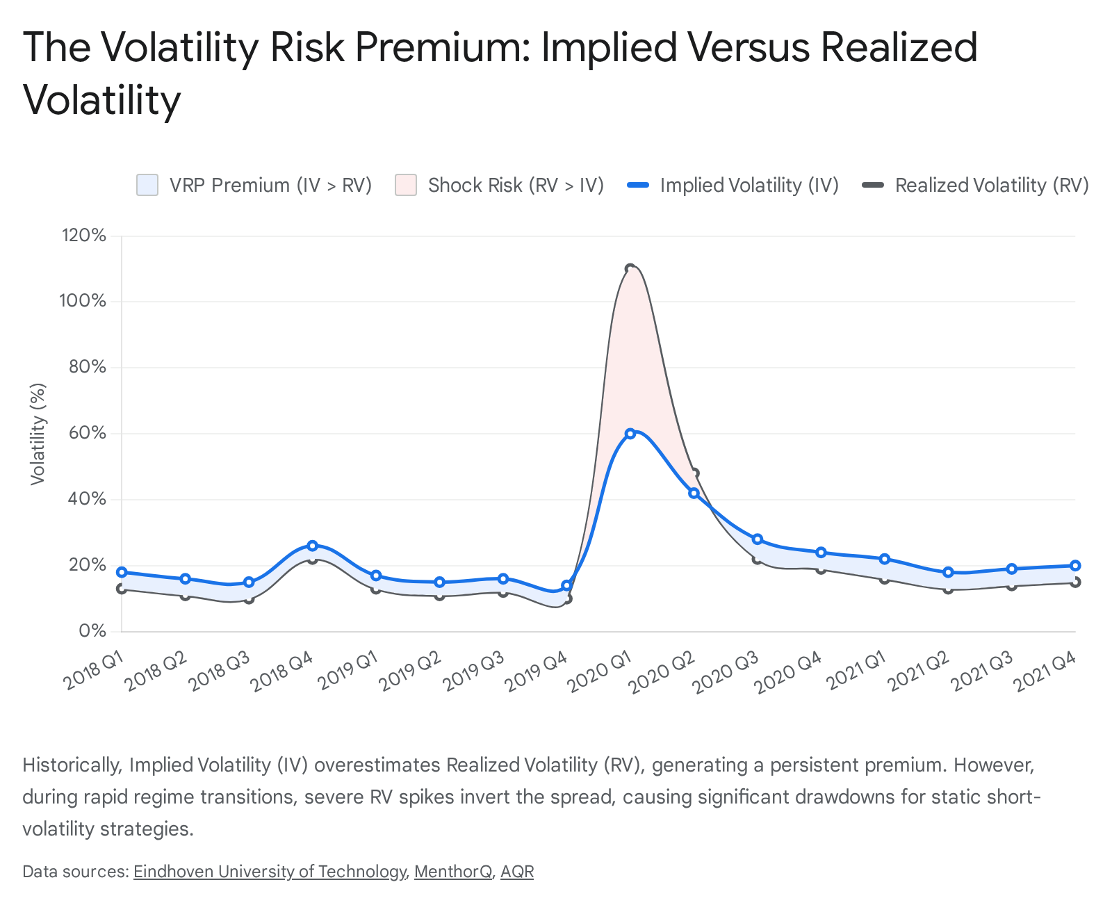
Implied Volatility (IV) represents the market's forward-looking forecast of future price movement, embedded directly into the pricing of option contracts 17. In contrast, Realized Volatility (RV) is a backward-looking metric measuring the actual historical variance of the underlying asset over a specific timeframe 17. Historically, market participants display a persistent behavioral bias: they consistently overestimate future risk. This systemic overestimation creates the Volatility Risk Premium (VRP) - a measurable, persistent spread where implied volatility generally trades at a premium to realized volatility 1819.
Swing strategies that systematically sell volatility (such as executing short straddles, iron condors, or delta-hedged short options) are designed to harvest this premium. These strategies tend to be highly profitable across both low-volatility environments and gradually declining equity regimes, provided that the daily realized volatility remains subdued 19. Even during mild bear markets, if the descent is orderly, the decay of the inflated option premium outpaces the directional losses, yielding positive returns 19. The profitability of these strategies is mathematically tethered to the spread between the locked-in IV at trade entry and the actual Forward Realized Volatility (FRV) that transpires during the life of the option contract 17.
Regime Shifts in Volatility and Tail Risk
The existential danger for swing traders utilizing short-volatility setups arises during rapid regime shifts - specifically, extreme, non-linear expansions in realized volatility. While selling premium during high-IV regimes yields mathematically higher absolute credits, executing these strategies blindly during periods of peak historical volatility expansion leads to catastrophic drawdowns 20.
During structural macroeconomic failures or geopolitical shocks, Forward Realized Volatility can massively exceed the elevated Implied Volatility, resulting in deeply negative spreads. For example, in early 2020 prior to the onset of the pandemic, implied volatility on crude oil was elevated at roughly 40%, making short-volatility trades appear highly attractive relative to recent historical norms 17. However, as the global economy halted, actual realized volatility exploded to over 140% 17. Traders who sold premium based on the IV-RV shortcut experienced massive losses as the FRV-IV spread inverted aggressively 17.
Optimal swing opportunities in the volatility space frequently materialize in a highly specific matrix condition: when implied volatility remains elevated due to lingering fear, but historical realized volatility has peaked and is beginning to contract 20. Recognizing this precise transition from a "Crisis" regime to a stabilizing environment allows systematic traders to capture elevated premiums before IV collapses to historical norms. Matrix analysis of regime combinations reveals that targeting environments where extreme implied volatility pairs with peak historical volatility expansion can result in significant average net gains (up to 46% historically in tested ETF straddle portfolios), provided the exact inflection point of the regime transition can be mathematically identified 20.
Furthermore, when constructing delta-hedged portfolios, the choice between using implied versus realized volatility as the input parameter is crucial. Academic studies demonstrate that IV-based hedging delivers more stable returns, lower return volatility, and superior risk mitigation 21. Because implied volatility is forward-looking and market-implied, it adapts more effectively to changing market conditions, improving delta accuracy and reducing the transaction costs associated with high-frequency rebalancing compared to backward-looking historical volatility metrics 21.
Cross-Asset Correlations and Structural Macro Shifts
Market regimes are not confined to the isolated price action of a single equity index; they represent profound systemic shifts in the covariance structure of global markets. Quantitative swing strategies heavily rely on asset diversification and stable correlation matrices to manage portfolio variance. When a macroeconomic regime undergoes a structural shift, historical correlations frequently break down, rendering carefully constructed cross-asset hedges entirely ineffective 22.
The Dissolution of Traditional Safe Havens
Historically, episodes of market stress were characterized by standard "risk-off" dynamics: equities declined, volatility surged, and fixed income assets rallied as capital sought a flight to safety. However, distinct underlying macroeconomic drivers can produce identical surface-level volatility but radically different correlation structures. For instance, the market regime of 2022 was driven by persistent, systemic inflation shocks rather than a standard credit crisis or liquidity event 23.
Consequently, the reliable historical negative correlation between equities and fixed income dissolved; both asset classes became positively correlated, declining simultaneously as global central banks aggressively raised interest rates to combat inflation 2324. This regime transition signifies a structural shift toward sustained, medium-term volatility where traditional safe havens fail to provide expected diversification 22. In these inflationary environments, cross-asset dependence strengthens, multiscale linkages intensify, and systemic risk migrates across asset classes rather than dissipating into non-correlated assets 2533.
During such systemic disruptions, swing traders utilizing cross-asset strategies must rely on advanced statistical models. Commodity hedging, traditionally viewed as a reliable defense mechanism, becomes highly regime-dependent. Studies applying Multifractal Detrended Cross-Correlation Analysis (MFCCA) and Generalized Orthogonal GARCH (GO-GARCH) frameworks reveal that while assets like gold and WTI crude oil maintain somewhat reliable hedging properties during crises, other commodities like wheat and natural gas exhibit highly unstable performance due to localized supply-side shocks 25. The GO-GARCH model is necessary in these regimes to accurately capture the asymmetric co-movements and volatility spillovers that ruin static correlation assumptions 25.
Interest Rate Regimes and Trend Following Efficacy
One of the most persistent and extensively studied systematic swing strategies is cross-asset trend-following, frequently deployed by Commodity Trading Advisors (CTAs). A common assumption within the financial industry is that the multi-decade success of trend-following was merely an artifact of a 40-year secular decline in global interest rates, which provided a persistent tailwind for fixed-income long positions 26.
However, deep historical backtesting extending over a century rigorously debunks this narrative. Data analyzing time-series momentum strategies all the way back to 1880 indicates that the efficacy of trend-following is not dependent on the absolute level or the directional vector of nominal interest rates 2627. Trend-following has maintained consistent profitability, strong risk-adjusted returns, and positive diversification characteristics during both protracted rising-rate regimes and sustained low-rate regimes 2627.
The strategy's defining structural advantage is its ability to dynamically switch from long to short positioning across equities, bonds, currencies, and commodities. This dynamism allows the strategy to exploit the persistent autocorrelation generated by monetary policy transitions and central bank interventions, regardless of whether those interventions involve hiking or cutting rates 2426. Data from the Bank for International Settlements (BIS) confirms that during periods of heightened interest rate volatility, hedging activity and cash-futures basis trades surge, bolstering trading volume in interest rate derivatives and providing ample liquidity for systematic trend followers to execute their models 28.
Microstructural Impacts of Algorithmic and High-Frequency Trading
The frequency, duration, and transition speed of market regimes have been permanently altered by the proliferation of Algorithmic Trading (AT) and High-Frequency Trading (HFT). By 2024, algorithmic platforms and AI-driven systems commanded massive global trading volumes - generating over $10.4 billion in revenue and projected to reach $16 billion by 2030 - fundamentally reshaping market microstructure, price discovery, and liquidity provision across North America, Europe, and the Asia-Pacific regions 293839.
In stable, low-volatility regimes, HFT algorithms provide a steady, continuous stream of limit orders to the market. This intense algorithmic participation narrows bid-ask spreads, drastically reduces transaction costs, and generally improves the informational efficiency of the market 40304243. By continuously executing complex statistical arbitrage and automated market-making strategies, these algorithms ensure that micro-pricing discrepancies are swiftly corrected 4344. For the retail or institutional swing trader, this liquidity abundance ensures optimal execution with minimal slippage upon entry and exit.
However, the liquidity provided by high-frequency market makers is notoriously fragile and highly regime-dependent. During periods of heightened information asymmetry, sudden macroeconomic shocks, or unexpected geopolitical news, risk-management algorithms are programmed to rapidly scale back trading activity or withdraw liquidity from the order book entirely 4030. This sudden, systemic absence of order book depth actively consumes liquidity just when it is needed most.
When liquidity evaporates, standard sell orders exacerbate downward momentum, triggering automated stop-loss cascades. Because algorithmic trading models frequently share similar data inputs, latency architectures, and risk management protocols, their concurrent reactions to market signals can induce artificial price spikes and create rapid, self-reinforcing feedback loops 304345. This dynamic was glaringly evident during the 2010 Flash Crash and subsequent modern micro-crashes 3042.
For the swing trader, the implications are severe: transitions between market regimes are no longer gradual, multi-day processes. The onset of a high-volatility regime can occur in milliseconds, easily bypassing static stop-loss limits and forcing massive slippage. The integration of advanced artificial intelligence and quantum-accelerated Monte Carlo simulations into these HFT risk engines ensures that algorithmic dominance will continue to compress the timeframes of regime shifts, necessitating that human swing traders rely on automated, implied-volatility-based hedging mechanisms rather than manual reaction times 2930.
Institutional Strategy Adaptation and the Quant Winter
The recent evolution of institutional systematic investing provides a clear roadmap for how swing strategies must adapt to survive aggressive regime shifts. The period from 2018 to 2020, widely referred to in the industry as the "Quant Winter," demonstrated the critical vulnerabilities of relying on static, classical academic factor models 4631.
During the Quant Winter, traditional quantitative equity factors - such as static Value and Momentum - suffered severe, prolonged drawdowns. Detailed analyses attribute this underperformance to adverse macroeconomic environments, shifting market regimes where historical data no longer predicted future outcomes, and massive factor crowding by institutional capital 463132. Models that mechanically bought undervalued stocks and sold overvalued ones, or that blindly chased medium-term momentum, were continuously whipsawed by erratic policy announcements and sudden reversals 4632.
Dynamic Factor Allocation and Machine Learning
In response to the failures of the Quant Winter, elite institutional quantitative funds have transitioned toward dynamic factor combination and highly adaptive, machine-learning-driven methodologies 3132. Rather than holding static, unyielding allocations to individual factors, top-performing funds leverage real-time regime classifications to aggressively rotate exposures. Recognizing that static approaches create systematic vulnerabilities during regime transitions, the industry has developed adaptive methodologies that respond instantly to shifting market volatility and macroeconomic indicators 31.
The success of these adaptive strategies was starkly evident in recent market cycles. For example, AQR Capital Management's flagship quantitative strategies posted robust double-digit returns in 2025, with its Apex multi-strategy fund returning 19.6% and its Helix trend-following strategy returning 18.6% 4933. AQR achieved this by blending classical, academic research-driven strategies with proprietary machine-learning approaches 4933. Crucially, the firm exhibited extreme mechanical discipline; when the momentum factor decayed on specific equities due to a regime shift, the algorithms mechanically slashed positions without emotional hesitation 49. This discipline proved that factor investing does not break permanently; rather, factors simply go out of favor during specific regimes, requiring the quantitative model to dynamically re-optimize 49.
Conversely, quantitative strategies that failed to evolve or that relied too heavily on slower, traditional trend-following models suffered immensely when sudden macroeconomic reversals occurred. In early 2025, Man Group's flagship AHL Diversified Programme and other quant strategies faced steep double-digit drawdowns as heightened market volatility and geopolitical uncertainty tested the resilience of their models 34. Sudden reversals across equities, bonds, and currencies caught slower trend-following models off guard, proving that algorithms built to follow patterns over several months struggle to pivot quickly enough in a whipsawing, mean-reverting environment 34.
To survive the modern landscape of high-frequency regime transitions, institutional models now incorporate real-time portfolio optimization that integrates non-traditional alternative data. This includes the natural language processing of central bank communications and earnings call transcripts, monitoring global supply chain indicators, and cross-asset signal integration 35. By anticipating regime shifts before they fully materialize in the price action, these dynamic models insulate the portfolio from the exact drivers that caused the historical Quant Winter.
Conclusion
The profitability and mathematical viability of swing trading strategies are fundamentally constrained by the active market regime. The quantitative evidence is definitive: technical indicators, stop-loss algorithms, and cross-asset correlation models do not possess universal, all-weather reliability. Instead, their statistical edge fluctuates drastically between trending, range-bound, and high-volatility states.
Trend-following tools and tight risk-management constraints excel strictly in regimes characterized by positive autocorrelation and sustained directional momentum. However, when markets inevitably compress into range-bound consolidation - which constitutes the majority of trading time - these exact tools generate rapid capital decay, necessitating a tactical shift toward mean-reversion oscillators and wider volatility parameters. Furthermore, the modern market microstructure, dominated by algorithmic liquidity provision, ensures that transitions between these regimes will be abrupt, volatile, and highly disruptive to static trading rules.
Successful swing trading, therefore, requires a complete departure from rigid heuristics. By integrating probabilistic regime detection models, continuously tracking the structural spread between implied and realized volatility, and dynamically adjusting execution parameters to the underlying statistical reality of the asset, systematic traders can mitigate mathematical decay. Adapting to the regime, rather than fighting it, allows market participants to exploit the distinct, shifting risk premiums offered across the full spectrum of global financial environments.