Backtest Overfitting and Trading Strategy Replication
Evolution of Quantitative Performance Metrics
The foundational framework for evaluating the performance of investment strategies rests on Modern Portfolio Theory, pioneered by Harry Markowitz in 1952, which posits that rational, risk-averse investors optimize their portfolios by focusing exclusively on the first two moments of the return distribution: mean and variance 1. Building upon this mean-variance optimization framework, William F. Sharpe introduced the Sharpe Ratio in 1966 to measure the expected differential return per unit of risk associated with an investment strategy 123. Calculated as the excess return of a portfolio over the risk-free rate divided by the standard deviation of those excess returns, the Sharpe Ratio quickly became the industry standard for assessing whether historical returns were the product of sound investment logic or excessive risk-taking 24.
Under traditional interpretations, an annualized Sharpe Ratio between 1.00 and 1.99 is considered robust, while a ratio exceeding 2.00 is highly exceptional, often prompting institutional scrutiny to verify whether leverage was heavily utilized 2. However, the standard Sharpe Ratio is constructed upon a set of rigid statistical assumptions that rarely hold true in modern financial markets. Specifically, the metric implicitly assumes that asset returns are independent and identically distributed (IID) and follow a perfect Gaussian (normal) distribution 156. Furthermore, the classical Sharpe Ratio evaluates the statistical significance of a strategy strictly in isolation, assuming that only a single hypothesis test has been conducted 356.
The advent of high-frequency market data, machine learning classification algorithms, and cloud-based parallel computing has rendered the single-trial assumption obsolete. Modern quantitative analysts routinely execute millions, or even billions, of backtest simulations to identify optimal parameter configurations across vast temporal and asset-class dimensions 147. Because the standard Sharpe Ratio point estimator lacks a mechanism to penalize the multiplicity of these trials, it systematically overstates the statistical significance of historical performance, creating an illusion of alpha that rapidly deteriorates in out-of-sample live trading environments 459.
Mechanics of Backtest Overfitting
To comprehend why machine learning and artificial intelligence trading strategies routinely fail to replicate their historical results, a strict distinction must be drawn between traditional model overfitting and backtest overfitting. In computer science and statistical learning, model overfitting occurs when an algorithm - such as a deep neural network or a random forest - memorizes the noise within a specific training dataset rather than capturing the underlying generative signal 108. This results in a model that performs flawlessly in-sample but fails to generalize to unseen out-of-sample data.
Conversely, backtest overfitting in mathematical finance is a manifestation of selection bias and the multiple testing problem 6109. It occurs during the strategy formulation process when a researcher evaluates a vast array of distinct models, parameter combinations, timeframes, and stop-loss rules on the same historical dataset, but only reports the performance of the single best-performing iteration 456.
Even if the researcher employs standard machine learning safeguards such as the hold-out method or out-of-sample validation periods, these techniques fail to identify backtest overfitting 6913. Each time an analyst evaluates a model's out-of-sample performance, modifies a parameter, and re-tests, the out-of-sample data effectively becomes integrated into the optimization loop, contaminating its independence 9. Because the signal-to-noise ratio in global financial markets is exceptionally low, testing thousands of non-predictive variations virtually guarantees the discovery of a strategy that exhibits a highly profitable historical equity curve purely by random chance 79. Under the influence of memory effects and non-stationary market regimes, such overfitted strategies do not merely generate random noise in live deployment; they systematically destroy capital 1314.
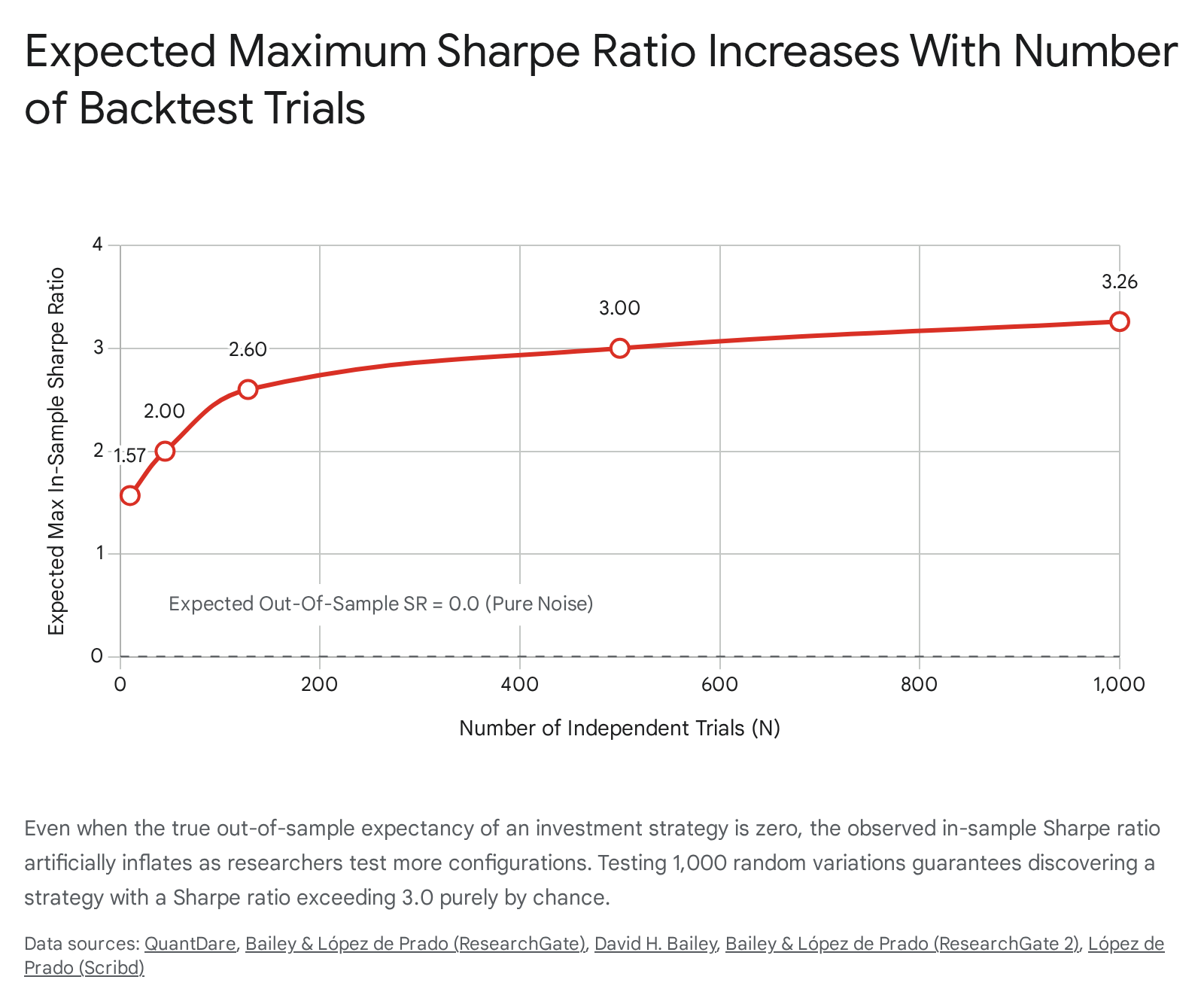
The False Strategy Theorem
The mathematical certainty of performance inflation under multiple testing is formalized in the False Strategy Theorem, established by David H. Bailey and Marcos López de Prado 1011. The theorem models the expected maximum in-sample Sharpe Ratio as a direct function of the number of independent strategy variations evaluated, demonstrating that a researcher can achieve any desired performance threshold simply by increasing computational output 131112.
The theorem operates under the null hypothesis that a set of proposed investment strategies possesses a true out-of-sample expected Sharpe Ratio of exactly zero 713. If a researcher evaluates $N$ independent strategy configurations, the in-sample Sharpe Ratio estimators follow a normal distribution due to the Central Limit Theorem 1420. The maximum of these normally distributed estimators follows a Gumbel extreme value distribution. Using this framework, the expected maximum in-sample Sharpe Ratio ($E[\max(\widehat{SR}_n)]$) can be analytically approximated.
The approximation integrates the variance across the estimated Sharpe Ratios of the trials ($V[{\widehat{SR}_n}]$), the Euler-Mascheroni constant ($\gamma \approx 0.5772$), the cumulative distribution function of the standard normal distribution ($Z$), and Euler's number ($e$) 1721. The mathematical formulation proves that the expected maximum Sharpe Ratio is strictly increasing with respect to the number of independent trials ($N$) and the variance of those trials 713.
The empirical consequences of this theorem reveal the severe fragility of unadjusted performance metrics. If an analyst conducts a skill-less brute-force search evaluating a rudimentary trading rule with merely seven binary parameters, they generate 128 independent trials ($2^7 = 128$). Purely through random variation, the expected maximum annualized Sharpe Ratio for the optimal iteration will exceed 2.6 15. Expanding this search space to 1,000 independent backtests mathematically guarantees an expected maximum Sharpe Ratio of approximately 3.26, despite the underlying strategy lacking any genuine predictive power 21.
Statistical Corrections for Selection Bias
To identify robust quantitative strategies and separate genuine empirical findings from statistical flukes, researchers require performance evaluation methodologies that actively control for both non-normal returns distributions and multiple testing inflation 179.
The Probabilistic Sharpe Ratio
The standard Sharpe Ratio fails to measure the inflationary effects generated by short sample lengths and non-Gaussian returns 710. Empirical financial time series are predominantly characterized by negative skewness - where large losses occur more frequently than large gains - and positive excess kurtosis, representing "fat tails" or a heightened probability of extreme outlier events 15. Because the variance of the Sharpe Ratio estimator increases substantially in the presence of negative skewness and positive kurtosis, point estimates derived from non-normal returns carry much wider confidence intervals 15.
To address this, Bailey and López de Prado developed the Probabilistic Sharpe Ratio (PSR), which establishes the probability that a strategy's true Sharpe Ratio exceeds a designated benchmark threshold 7. The PSR framework integrates the strategy's track record length ($T$) alongside the empirical skewness ($\hat{\gamma}_3$) and kurtosis ($\hat{\gamma}_4$) of the returns distribution 7. By adjusting the standard error of the Sharpe Ratio using these higher moments, the PSR delivers a calibrated confidence level 57. Consequently, two strategies that display an identical nominal Sharpe Ratio of 1.50 will yield vastly different PSR confidence intervals if one strategy generates normally distributed returns while the other achieves its returns through highly skewed, tail-risk exposures 1.
The Deflated Sharpe Ratio
While the PSR successfully calibrates a strategy's statistical significance against its returns distribution, it operates under the assumption that only a single strategy was tested 67. To resolve the multiple testing problem, Bailey and López de Prado introduced the Deflated Sharpe Ratio (DSR) 6710.
The DSR is mathematically structured as a Probabilistic Sharpe Ratio wherein the static rejection threshold is replaced by a dynamic, selection-bias-aware threshold 57. This dynamic benchmark is precisely the expected maximum Sharpe Ratio derived from the False Strategy Theorem 57. The framework integrates five distinct variables to deflate the nominal metric: the track record length, the skewness of returns, the kurtosis of returns, the variance across the estimated Sharpe Ratios of all trials conducted, and the number of independent trials ($N$) 710.
A critical operational requirement for applying the DSR is the precise recording of all historical backtests to determine the true value of $N$ 21. Because quantitative algorithms often execute highly correlated variations of the same core strategy (e.g., tweaking a moving average from 50 days to 51 days), the raw number of total backtests ($M$) overstates the true breadth of the search space. Researchers typically estimate the effective number of independent trials ($N$) using dimension-reduction clustering protocols based on the average correlation matrix of the trial return streams 102115.
When applied rigorously, the DSR outputs the true probability that a data-mined strategy is not merely an artifact of optimization. A DSR output below 0.5 indicates performance indistinguishable from pure chance; an output near 0.8 suggests the presence of a weak signal; and a DSR exceeding 0.95 is generally required to reject the null hypothesis and confirm the existence of a robust statistical edge 5.
Minimum Backtest Length Limitations
The mathematical relationship between the number of trials and the expected inflation of performance metrics establishes strict boundaries on sample sizing, quantified as the Minimum Backtest Length (MinBTL) 61215. The MinBTL defines the absolute minimum duration of historical data required to ensure that the expected maximum in-sample Sharpe Ratio does not fully deviate from the expected out-of-sample performance 6131523.
The required sample length scales logarithmically relative to the number of independent trials executed 1315. The upper bound of the MinBTL formula dictates that the required years of historical data must be approximately greater than $2 \ln(N)$ divided by the square of the expected maximum Sharpe Ratio 1315. If an analyst lacks sufficient historical data to meet the MinBTL requirement for their specified search space, any resulting high-performance strategy is statistically invalid, irrespective of its nominal metrics 1420.
| Independent Strategy Trials ($N$) | Theoretical Max In-Sample Sharpe Ratio | Approximate Minimum Backtest Length Required |
|---|---|---|
| 1 Trial | N/A (Standard Evaluation) | N/A |
| 7 Trials | 1.00 | ~2.0 Years |
| 10 Trials | 1.57 | ~2.5 Years |
| 45 Trials | 1.00 (At fixed threshold) | ~5.0 Years |
| 128 Trials | 2.60 | ~8.0 Years |
| 1,000 Trials | 3.26 | ~15.0+ Years |
Table 1: Approximate mathematical relationship between the volume of independent computational trials, the artificial inflation of expected in-sample Sharpe Ratios (assuming an out-of-sample expectancy of zero), and the requisite Minimum Backtest Length necessary to preserve statistical validity 1313202115.
As demonstrated by the parameters of the theorem, an analyst processing 45 independent model configurations using only five years of historical data is mathematically destined to identify an overfitted strategy that reports an annualized Sharpe Ratio of 1.0, but which will yield zero return out-of-sample 1315. Consequently, researchers must carefully constrain their parameter optimization processes to avoid exceeding the statistical capacity of their available historical data 21.
Academic Critiques of Conservative Adjustments
While the Deflated Sharpe Ratio and associated multiple testing corrections provide vital defense mechanisms against data mining, the framework has drawn targeted critiques regarding the severity of its statistical penalties 16. In global equity and derivatives markets, structural inefficiencies and true signal-to-noise ratios are innately low; consequently, aggressive mathematical deflation can easily obscure genuine, albeit weak, financial signals 917.
A primary objection is that stringent frameworks like the DSR induce significant Type II errors - the false rejection of valid, profitable investment algorithms 1216. Critics argue that utilizing uniformly harsh thresholds fails to accommodate the nuances of specific market microstructures and leads to the discard of strategies that exhibit episodic drawdowns but ultimately retain long-term positive expectancy 17. Within the broader literature of financial econometrics, Levi and Welch (2017) have articulated analogous concerns regarding hyper-conservative statistical adjustments, demonstrating that standard industry beta shrinkage models and conservative cost-of-capital estimates often obfuscate accurate risk-reward profiles by aggressively muting empirical variation 18192021.
Further complicating the assumption that all data-mined strategies are functionally void, empirical investigations utilizing empirical Bayes (EB) mining have demonstrated resilience in naively optimized parameters. Research evaluating thousands of stock predictors revealed that constructing portfolios based purely on the top 1% of historically observed, unadjusted Sharpe Ratios continued to yield an out-of-sample Sharpe Ratio of 1.45, performing comparably to heavily vetted anomaly strategies published in tier-one financial journals 30. These findings imply that while the False Strategy Theorem mathematically holds for perfectly random data, actual financial time-series contain persistent autocorrelation and structural anomalies that can occasionally survive brute-force selection processes without total out-of-sample decay 3022.
To balance this tension, some quantitative architects advocate against optimizing exclusively for a single risk-adjusted point estimator. By disaggregating complex models - for example, deploying one classifier strictly to predict trade direction (side) and an independent regression model to estimate position conviction (size) - researchers can prioritize the F1-score (harmonic mean of precision and recall) over the Sharpe Ratio, thereby retaining responsive strategies that might otherwise be filtered out by conservative deflation algorithms 17.
Machine Learning Vulnerabilities in Market Environments
As quantitative finance increasingly transitions from simple parametric rulesets to high-dimensional machine learning frameworks, the mechanisms of strategy failure have evolved 232425. Advanced classification algorithms, such as Random Forests and Long Short-Term Memory (LSTM) neural networks, possess immense capacity to detect non-linear dependencies across thousands of technical indicators 243536. However, this capacity simultaneously makes them uniquely vulnerable to environmental non-stationarity 372627.
Machine learning trading strategies frequently exhibit spectacular backtest profiles that instantly collapse upon live deployment 93528. Empirical validation studies repeatedly highlight this discrepancy. In a 2026 academic study spanning three years of Nifty 50 index data, researchers constructed a Random Forest model utilizing 17 technical indicators. While the model achieved a flawless 100% training accuracy in-sample, its out-of-sample live accuracy deteriorated to 50% 35. Crucially, because the algorithm optimized for high-frequency signal generation based on lagging public data, the integration of a standard 0.2% round-trip transaction cost devastated its equity curve, yielding a net absolute return of merely 5.34% over 50 trades - severely underperforming a basic 55.02% passive buy-and-hold benchmark 35.
Similar limitations manifest in deep learning time-series forecasting. A study applying LSTM networks to intraday gold (XAUUSD) trading discovered that combining the neural network with technical indicators (SMA, MACD, Bollinger Bands) produced a commanding backtest Sharpe Ratio of 2.51 and a 38.4% win rate 36. Yet, forward-testing the identical architecture in live market conditions revealed zero strategies with positive mathematical expectancy, as the indicator rankings from the backtest failed to transfer robustly to unseen data 36.
These failures emphasize that optimizing machine learning models against historical snapshots fundamentally assumes the future will structurally resemble the past 37. In reality, financial markets undergo continuous volatility regime shifts, correlation breakdowns, and behavioral adaptations driven by macroeconomic events 3728. Models that lack persistent memory architecture or adaptive contextual reasoning often become hopelessly brittle during regime transitions, optimizing for trending behaviors precisely as the market enters a period of high-noise consolidation 3728.
Artificial Intelligence and Large Language Model Forecasting
The deployment of generative Artificial Intelligence, particularly Large Language Models (LLMs), has introduced unprecedented capabilities in financial sentiment analysis, automated reasoning, and unstructured data processing 4142. By autonomously interpreting earnings transcripts, global news flows, and geopolitical developments, LLMs operate fundamentally differently than numerical, rules-based algorithms 4142. Consequently, they generate novel backtesting paradoxes that completely bypass the statistical checks of the Deflated Sharpe Ratio 29.
Data Leakage and the Eradication of True Out-of-Sample Testing
The single greatest impediment to evaluating LLM-based trading strategies is the impossibility of ensuring temporal isolation 29. Traditional statistical models initialize with blank parameters and learn exclusively from the historical data provided 9. In stark contrast, an LLM possesses vast, generalized world knowledge baked directly into its neural weights during pre-training 29.
If a quantitative team attempts to backtest an LLM agent on market events from 2023, but the underlying base model was trained on corpora extending into 2024, the agent implicitly possesses "future" knowledge regarding corporate bankruptcies, interest rate decisions, and broad market trajectories 29. This absolute look-ahead bias completely invalidates the backtest 2945. Furthermore, efforts to restrict the LLM by utilizing date-filtered web searches (e.g., instructing the agent to only read news from before a specific date) remain structurally flawed; search engine algorithms, result snippets, and subsequently updated web pages effortlessly leak future information back into the context window 29.
To conduct viable strategy evaluations with LLMs, researchers must utilize models with strict, documented knowledge cutoffs, creating a narrow validation window extending from the cutoff date to the present 29. Additionally, the research phase must rely on "time-capsule" data architecture - scraping and locally storing tens of thousands of URLs precisely as they existed on the target historical date, thereby forcing the AI agent to query an isolated, static corpus rather than the live internet 29. As commercial LLM providers increasingly shift toward "continual learning" models that update continuously based on real-time data streams, deterministic historical backtesting of AI agents will become functionally impossible 29.
Label Bias and Evaluator Self-Preference
Compounding the issue of temporal leakage are the intrinsic cognitive biases displayed by LLMs during decision-making tasks 423031. Extensive empirical testing reveals that foundational models exhibit pronounced label bias, systematically favoring specific categorical answers regardless of the empirical input, often mirroring the semantic prejudices of their training data 4230. When analyzing scientific or complex financial summaries, modern LLMs demonstrate a high propensity for generalization bias, producing broad, oversimplified conclusions that mask the nuanced risk parameters of the underlying data 31.
These vulnerabilities are magnified when LLMs are integrated into Retrieval-Augmented Generation (RAG) frameworks to autonomously generate, rank, and evaluate trading hypotheses 32. Recent AI evaluation studies document a severe self-preference bias, wherein LLM judges systematically assign higher quality ratings, accuracy scores, and strategic validity to content generated by themselves (or models of similar architecture) over objectively superior human-authored baselines 3249. If an automated quantitative pipeline relies on an LLM to self-evaluate the backtested performance of its own logic, this self-enhancement loop creates an illusion of high strategic conviction, shielding fundamentally flawed strategies from objective risk management 3249.
Empirical Discrepancies in Live Deployment
The theoretical vulnerabilities of LLM-based financial strategies are distinctly visible in cross-sectional empirical studies spanning the 2023 - 2025 technology cycles 413334. While narrow, short-term evaluations often report significant AI outperformance, rigorous, long-term testing reveals severe performance degradation 4133.
To assess the generalizability of LLM market-timing strategies, researchers developed the FINSABER framework, evaluating AI agent performance across 100+ stock symbols over a two-decade simulation to explicitly control for survivorship bias and data-snooping 4133. The systematic backtests revealed that previously reported LLM advantages collapsed under broader cross-sectional evaluation 4133. Crucially, market regime analysis demonstrated that LLM strategies lack dynamic adaptivity: they act overly conservative during extended bull markets - consistently trailing passive benchmarks - and become overly aggressive in bear markets, incurring catastrophic drawdowns 4133.
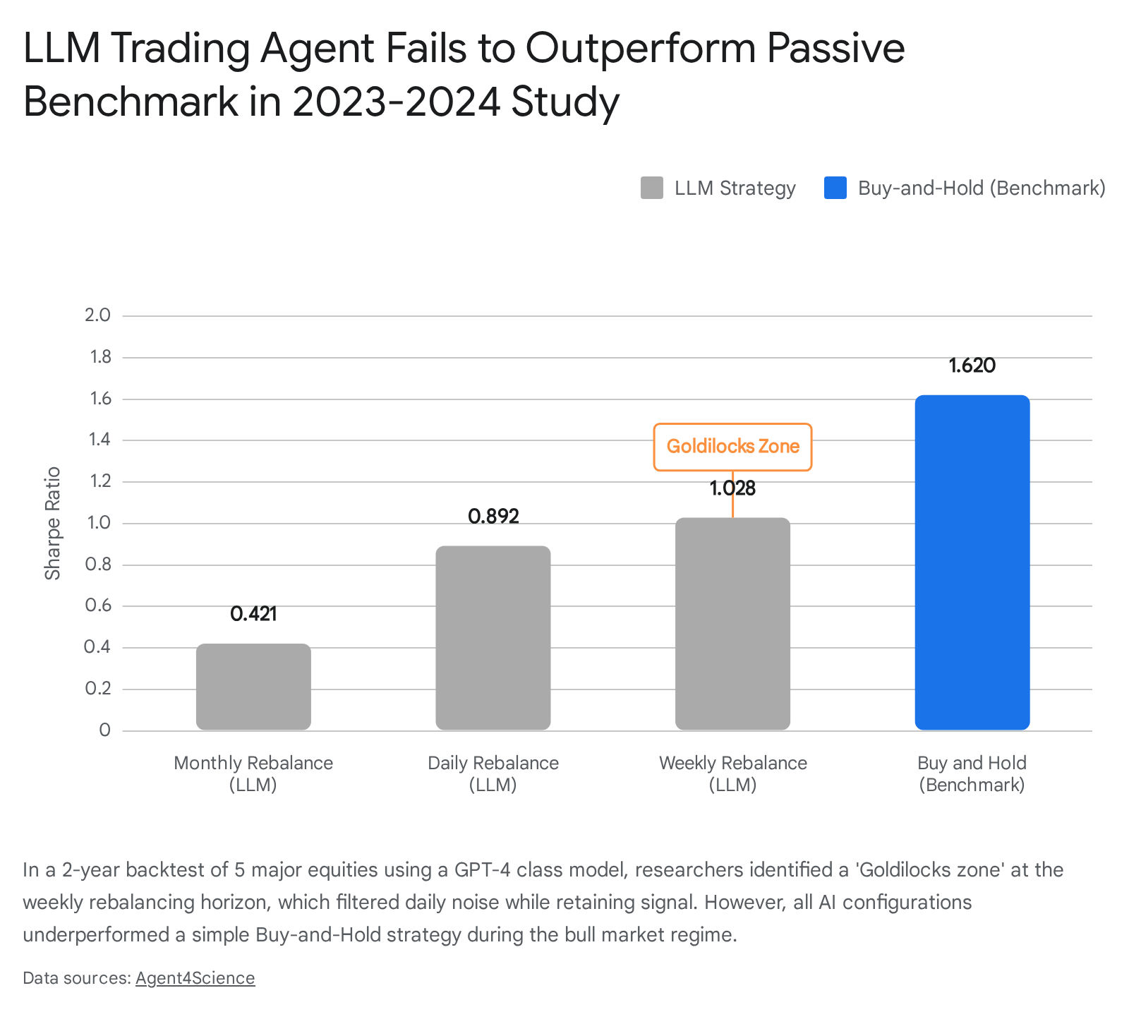
Further confirming these limitations, a 2026 study isolated the impact of trading frequency on LLM decision-making using a GPT-4 class agent across five major technology equities over the 2023 - 2024 bull market 52. The experiment sought to determine the optimal rebalancing horizon by analyzing daily, weekly, and monthly AI executions 52.
The findings indicated a structural "Goldilocks zone" for LLMs: a weekly rebalancing schedule yielded an optimal Sharpe Ratio of 1.028, effectively filtering the noise inherent in daily rebalancing (Sharpe 0.892) while preventing the signal decay suffered in monthly rebalancing (Sharpe 0.421) 52. However, despite optimal frequency calibration, no AI variation managed to outperform a simple Buy-and-Hold benchmark, which commanded a Sharpe Ratio of 1.620 over the identical period, underscoring the models' failure to capture sustained directional momentum 52.
Survivorship Bias and Execution Slippage
When transitioning AI strategies from research environments to live capital deployment, mechanical execution realities frequently destroy theoretical alpha 2428. Researchers commonly utilize sanitized price series that silently remove assets delisted due to bankruptcy or acquisition 2841. By training exclusively on survivors, AI algorithms learn solely from the structural patterns of successful entities 2841. Upon live execution, when the agent inevitably interacts with a distressed asset exhibiting deteriorating bid-ask spreads, it applies winner-based logic to a failing instrument, resulting in immediate catastrophic losses 28.
Compounding survivorship bias is the pervasive mismodeling of execution slippage. Basic backtesting architecture assumes instantaneous order fulfillment at the precise mid-price observed when the trading signal fired 28. In physical markets, acquiring inventory requires crossing the spread via market orders, incurring immediate friction 2428. For strategies utilizing leverage, rapid turnover, or complex multi-leg derivatives, this execution slippage transforms ostensibly high-Sharpe algorithms into capital incinerators 242853. A documented empirical test of an LLM crypto-trading bot revealed that high-frequency, highly-leveraged configurations bled 15.2% of total equity to trading costs and slippage in merely two weeks, highlighting that theoretical intelligence cannot overcome structural market friction 53.
Institutional Validation Frameworks
To mitigate the systemic failures of machine learning and generative AI models, institutional quantitative funds deploy advanced validation pipelines that extend beyond basic point-estimator corrections 1228.
Standard out-of-sample hold-out methodology and k-fold cross-validation are deeply flawed when applied to financial time series, as they frequently leak temporal information from the test set back into the training logic 81245. To combat this, institutions utilize Combinatorial Purged Cross-Validation (CPCV). CPCV architecture systematically generates exact combinations of training and testing arrays while ruthlessly purging any training observations that overlap with or contain leaked temporal data from the testing periods, ensuring true out-of-sample integrity 12.
Furthermore, robust institutional architecture demands dynamic regime awareness. Rather than running a static AI model universally across all market phases, funds segment historical data into discrete regimes based on realized volatility (e.g., low, elevated, extreme) 3728. Distinct models are trained exclusively on data reflecting their assigned regime. In live execution, a supervisory volatility-gating layer continuously monitors macroeconomic conditions and dynamically routes trade generation to the specific AI model calibrated for the current environment 28. By combining regime-aware architecture, realistic fill-decay simulation, and stringent multiple-testing corrections like the Deflated Sharpe Ratio, quantitative researchers can systematically differentiate between durable investment logic and transient statistical mirages.