LSTM and recurrent networks for stock price forecasting
The application of deep learning to financial time-series forecasting has become a central focus within quantitative finance and artificial intelligence research. Among the various architectures deployed over the past decade, the Long Short-Term Memory (LSTM) network has emerged as a predominant methodology. This prominence is driven by the network's theoretical capacity to model complex, non-linear dependencies over extended temporal sequences without succumbing to the mathematical decay that plagues simpler recurrent models. Financial markets generate immense volumes of sequential data - ranging from daily closing prices and trading volumes to microsecond-level limit order book states and macroeconomic indicators - that theoretically align with the sequence-to-sequence processing strengths of recurrent architectures 12.
However, a critical and exhaustive review of the empirical evidence reveals a substantial disconnect between the academic claims of predictive accuracy and the practical realities of algorithmic trading and portfolio management. While numerous peer-reviewed studies report extraordinarily low error rates and high directional accuracy using LSTM networks, quantitative practitioners, institutional researchers, and rigorous replication studies frequently identify these published results as artifacts of systemic methodological flaws 142. Issues such as the predictive lag illusion, temporal data leakage through improper normalization, survivorship bias, and the pervasive omission of market frictions (such as transaction costs, slippage, and market impact) invalidate a significant portion of the literature 137.
This comprehensive report evaluates the evidence surrounding LSTM networks in stock-price forecasting. It dissects their architectural mechanisms, compares their empirical performance against both classical econometric models and newer attention-based frameworks, and examines the geographic disparities in their efficacy across developed and emerging markets. Furthermore, the analysis explores the systemic evaluation flaws that obscure the true financial utility of these models, ultimately defining the necessary conditions under which recurrent networks can contribute to viable trading strategies.
Architectural Foundations of Recurrent Networks
To contextualize the application of LSTMs in financial forecasting, it is necessary to examine the foundational architectural mechanisms that distinguish them from traditional statistical frameworks and standard feed-forward neural networks.
Mechanisms of Sequential Processing
Traditional feed-forward artificial neural networks process input features independently, utilizing no internal memory state. This renders them structurally incapable of retaining historical context, making them sub-optimal for time-series data where the sequence of events carries fundamental predictive value. Recurrent Neural Networks (RNNs) address this limitation by introducing cyclic connections into the network architecture, allowing information to persist across sequential time steps 45.
However, standard RNNs suffer from significant mathematical limitations during the training phase, specifically the vanishing and exploding gradient problems. When backpropagating errors through long temporal sequences, the gradients used to update the network weights either diminish toward zero or grow exponentially 4. This prevents standard RNNs from learning long-range dependencies, restricting their effective memory to only the most recent time steps.
Long Short-Term Memory networks were specifically engineered to solve this limitation. The architecture utilizes a complex cellular state governed by three distinct regulatory gates 56: 1. The Forget Gate: Determines the specific information from the previous cell state that should be discarded or retained based on the current input. 2. The Input Gate: Identifies new information from the current time step that holds predictive value and should be integrated into the cell state. 3. The Output Gate: Computes the hidden state for the subsequent time step based on a filtered version of the updated cell state.
This sophisticated gating mechanism theoretically allows the LSTM to retain relevant historical data - such as long-term macroeconomic shifts, previous earnings surprises, or prolonged volatility regimes - over arbitrary intervals, while actively filtering out high-frequency daily market noise 2. In the context of equity markets, this capability is highly sought after, as financial time series exhibit both long-term momentum and short-term mean reversion 712.
Handling the Characteristics of Financial Time Series
Financial time series data is notoriously challenging to model. It is characterized by an exceptionally high noise-to-signal ratio, non-stationarity, heteroskedasticity (volatility clustering), and extreme susceptibility to exogenous shocks 1. Standard econometric models, such as the Autoregressive Integrated Moving Average (ARIMA) or Generalized Autoregressive Conditional Heteroskedasticity (GARCH), rely heavily on mathematical assumptions of linearity and stationarity. When these assumptions are violated by real-world market dynamics, traditional models struggle to adapt 713.
Deep learning models like LSTMs operate as universal function approximators capable of capturing intricate, non-linear mappings between high-dimensional feature spaces and future price movements without requiring strict statistical assumptions about the underlying data distribution 1415. This flexibility has driven their widespread adoption in quantitative finance. Researchers utilize LSTMs to model the fat-tailed return distributions and sudden regime shifts inherent in global equity markets, theorizing that the neural network can identify latent factors and hidden market states that evade classical linear regression 715.
The Predictive Lag Illusion and Baseline Failures
Despite the theoretical alignment between LSTM architecture and financial time series, the empirical application often yields deceptive results. The most pervasive and critical flaw in univariate LSTM stock forecasting is the phenomenon known as the "lag illusion," or the persistence model fallacy.
The Mechanics of the Lag Illusion
Financial time series, particularly in highly efficient markets like the United States, closely approximate a random walk. In a near-random walk environment, the most mathematically robust predictor of tomorrow's price is simply today's closing price. When an LSTM network is trained on raw, non-stationary closing prices with an objective function designed to minimize the Mean Squared Error (MSE), the optimization algorithm rapidly identifies this property 1.
Because financial data contains massive amounts of noise, attempting to predict an actual trend reversal carries a high penalty if the model is incorrect. To minimize the average error penalty across thousands of training epochs, the neural network converges on a local minimum: the persistence strategy. The model learns to output $P_{t+1} \approx P_t$.
When researchers plot the predicted price curve against the actual historical price curve, the two lines appear virtually identical, frequently leading to claims of high predictive accuracy 1. However, microscopic examination of the individual data points reveals that the predicted curve is simply the actual historical curve shifted horizontally by one temporal unit.
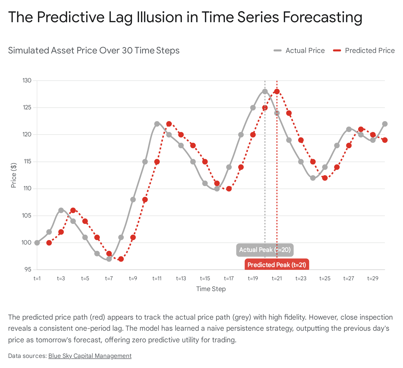
The implications of the lag illusion are profound. A model exhibiting this behavior will record highly favorable statistical metrics, such as a high $R^2$ coefficient and low Root Mean Square Error (RMSE) 1. These metrics trick researchers lacking deep financial domain expertise into believing the network has uncovered underlying market dynamics. In reality, the LSTM possesses absolutely zero predictive ability; it relies entirely on retroactive data 1. A trading strategy executing orders based on a persistence model will systematically execute trades one day late, resulting in consistent capital destruction when exposed to live markets.
Statistical Versus Financial Evaluation Metrics
A fundamental critique of LSTM research in stock-price forecasting is the profound and systemic disconnect between the statistical metrics used to train and evaluate the models in computer science, and the financial metrics required to validate a trading strategy's real-world viability in quantitative finance.
Limitations of Statistical Accuracy Measures
Machine learning models inherently rely on mathematically differentiable loss functions to optimize their internal weights during backpropagation. Consequently, the vast majority of academic papers report final performance using statistical error metrics such as Mean Squared Error (MSE), Root Mean Square Error (RMSE), Mean Absolute Error (MAE), and Mean Absolute Percentage Error (MAPE) 1617.
While essential for algorithmic convergence, these metrics are fundamentally inadequate for evaluating financial utility:
- RMSE and MSE: By squaring the differences between predicted and actual values, these metrics disproportionately penalize large deviations 16. While mathematically useful for gradient descent, an isolated low RMSE does not convey whether the model correctly predicted the direction of the price movement. If a stock surges by 5%, and the model predicted a 1% decline, the financial result is a total failure, yet the absolute squared error might remain small relative to the overall dataset scale 1618.
- MAE: This metric provides a linear penalty for errors, offering a more interpretable average magnitude of deviation (e.g., forecasting an average error of $1.50 per share) 17. However, like RMSE, it fails to evaluate whether the capital deployed based on the forecast would yield a positive return.
- MAPE: Expressing errors as a percentage is highly useful for cross-asset comparisons across different price scales. However, MAPE is highly sensitive to values approaching zero, which causes the metric to generate extremely large or undefined errors 19. Furthermore, its mathematical structure inherently favors models that underestimate rather than overestimate, introducing a systemic downward bias in forecasting 1719.
Requirements for Financial Utility Evaluation
In algorithmic trading, raw forecasting accuracy is secondary to risk-adjusted profitability. A model capable of predicting the exact price of an asset 90% of the time is useless if the 10% of incorrect predictions result in catastrophic capital loss. Rigorous financial evaluation requires metrics that account for capital allocation, risk exposure, downside volatility, and equity curve trajectory.
- Sharpe and Sortino Ratios: The Sharpe ratio measures the excess return of a strategy per unit of volatility 48. A model with high predictive accuracy that generates highly volatile, erratic returns may have a lower Sharpe ratio than a statistically less accurate but more consistent model. The Sortino ratio further refines this by penalizing only downside volatility, aligning more closely with actual investor risk tolerance 9.
- Maximum Drawdown (MDD): This represents the maximum observed capital loss from a peak to a subsequent trough before a new high is achieved. MDD is critical in live deployment because severe drawdowns can trigger institutional margin calls, mandate risk-management liquidation, or cause investor capitulation, rendering a technically accurate model practically unusable 42.
- Directional Accuracy (Hit Rate): The percentage of time the model correctly forecasts the binary direction (up or down) of the asset. In finance, a model with a mere 52% directional accuracy can be highly profitable if combined with a robust risk management system where the magnitude of correct predictions (win size) significantly exceeds the magnitude of incorrect predictions (loss size) 18.
A comprehensive systematic review of 22 recent deep learning papers focused on stock market prediction revealed a stark methodological gap in the literature: only five studies reported finance-aware metrics like net profit or the Sharpe ratio, and zero studies reported the maximum drawdown 2. This systemic reliance on pure statistical accuracy severely limits the credibility and commercial viability of published LSTM frameworks, leaving their practical impact entirely unsubstantiated.
Comparison of Evaluation Metrics
| Metric Category | Metric Designation | Primary Analytical Function | Critical Limitations in Financial Context |
|---|---|---|---|
| Statistical | Root Mean Square Error (RMSE) | Penalizes large deviations; standard optimization target. | Fails to indicate directional accuracy; heavily distorted by outlier market shocks 1617. |
| Statistical | Mean Absolute Error (MAE) | Measures average absolute magnitude of forecast error. | Treats all directional errors linearly; provides no insight into deployed capital risk 17. |
| Statistical | Mean Absolute Percentage Error (MAPE) | Measures percentage error for normalized cross-asset comparison. | Generates undefined values near zero; mathematically biases toward under-forecasting 19. |
| Financial | Sharpe Ratio | Measures risk-adjusted excess returns over a risk-free rate. | Assumes normal distribution of returns, which financial markets routinely violate via fat tails 48. |
| Financial | Maximum Drawdown (MDD) | Measures the largest peak-to-trough realized capital loss. | A strictly historical measure; does not predict susceptibility to future systemic shocks 42. |
| Financial | Directional Accuracy | Measures frequency of correctly predicting positive or negative movement. | Does not account for the magnitude of the move; requires strict combination with win/loss ratios 218. |
Systemic Methodological Flaws in Research Design
When quantitative hedge funds and independent researchers attempt to replicate the highly optimistic findings published in computer science journals, the LSTM models almost universally fail to generate alpha. This failure is largely attributable to severe, often inadvertent, methodological errors in experimental design, specifically regarding data leakage, temporal validation, and survivorship bias.
Temporal Data Leakage and Normalization Errors
Data leakage occurs when information from outside the designated training dataset is inadvertently used to create the model, resulting in an artificially inflated and overly optimistic performance estimate. In financial deep learning, this most commonly manifests through improper data scaling and normalization procedures 1023.
Neural networks, particularly recurrent architectures utilizing sigmoid and tanh activation functions, require scaled inputs (typically normalized to values between 0 and 1, or standardized to a mean of zero and unit variance) to ensure gradient convergence. A pervasive error in academic literature is the application of min-max scaling or global z-score normalization to the entire historical dataset prior to executing the train-validation-test split 1023. By doing so, the global maximum and minimum prices - including extreme highs or lows that occur strictly in the future test set - are integrated into the scaling parameters used during training. The LSTM inadvertently gains implicit access to future market boundaries 23.
To rigorously prevent this form of look-ahead bias, normalization parameters must be fitted exclusively on the historical training window, and those exact parameters must subsequently be applied to transform the validation and test sets 1023. More advanced methodologies deploy rolling-window feature-wise z-score normalization to ensure zero cross-temporal leakage 11.
Validation Strategies: Cross-Validation Versus Walk-Forward
The standard methodology for evaluating machine learning models in non-sequential domains is k-fold cross-validation, which involves randomly partitioning the dataset into distinct subsets. Applying random k-fold cross-validation to financial time series is mathematically disastrous. Random shuffling destroys temporal continuity and explicitly trains the model on future data to predict past data 1213.
Robust financial machine learning mandates chronological walk-forward validation (utilizing expanding or rolling windows). In this framework, the model is trained on a historical window (e.g., Year 1 to Year 5), validated on the immediate subsequent period (Year 6), and tested on the following period (Year 7). The window then shifts forward. This simulates the exact real-world information flow an investor experiences, ensuring the model never sees future variance or regime shifts before making a prediction 41213.
Survivorship Bias and Universe Selection
Another systemic flaw undermining the literature is survivorship bias. Academic studies frequently evaluate LSTM models by selecting the current constituents of major indices (e.g., the current S&P 500, NASDAQ 100, or IDX30) and fetching their historical data spanning ten to twenty years 41218.
This approach inherently excludes all companies that went bankrupt, were delisted, or were acquired during that period. Training a model exclusively on an asset universe that is known in hindsight to have survived and thrived artificially inflates predictability, eliminates downside tail risk, and drastically overstates historical returns 418. Realistic quantitative evaluation requires point-in-time constituent databases to ensure the LSTM is tested against the exact opportunity set available to an investor on any specific historical date, including companies that eventually collapsed to zero.
Trading Frictions: Transaction Costs, Slippage, and Market Impact
Assuming an LSTM model avoids the lag illusion and is validated without data leakage, its transition from a theoretical academic construct to a deployable algorithmic trading strategy is immediately obstructed by market frictions. The academic literature overwhelmingly reports pre-cost gross returns, neglecting the fundamental realities of executing trades in live markets 213.
The Erosion of Alpha via Transaction Costs
LSTMs, particularly those analyzing daily or intraday high-frequency data, frequently identify short-term mean-reversion or momentum patterns that require high-turnover trading. If a model dictates frequent portfolio rebalancing or daily long-to-short positional flips, the accumulated explicit transaction costs (brokerage commissions, exchange fees, and regulatory fees) will rapidly erode gross profits 814.
Research assessing multifactor timing strategies utilizing machine learning explicitly demonstrated this vulnerability. When simulating transaction costs ranging from a highly optimistic 1 basis point to a more realistic 14 basis points, the profitability of standard neural network models degraded substantially 8. Furthermore, an LSTM model boasting a seemingly robust 55% directional accuracy will consistently lose capital if the expected signal magnitude (the average percentage profit per winning trade) does not exceed the round-trip execution costs 18. Incorporating transaction costs into the evaluation often reveals that deep learning models generate returns inferior to simple buy-and-hold benchmarks 15.
Implicit Costs: Slippage and Market Impact
Beyond explicit commissions, algorithmic trading is heavily constrained by implicit execution costs: slippage and market impact. Slippage is defined as the price displacement between the moment an LSTM generates a trading signal and the moment the order is actually executed by the exchange 728. In fast-moving, volatile markets, the computational latency required to run a deep learning inference pipeline, combined with network routing delays, ensures that the optimal entry price may no longer exist 2829.
Executing significant trading volume introduces market impact, which is separated into temporary and permanent components. If an LSTM signals a high-conviction "buy" and places a large market order, it will consume the available liquidity in the limit order book. This pushes the execution price higher (temporary impact) and provides informational signaling to other algorithmic market participants (permanent impact) 714.
Studies investigating deep learning applications directly on high-frequency Limit Order Book (LOB) data, such as the DeepLOB framework, note that while models can forecast mid-price movements accurately, their practical trading power drops precipitously when accounting for tick sizes, queue positioning, and spread distributions 11. A highly accurate forecast of a micro-price movement is mathematically un-tradeable if the forecasted move is smaller than the bid-ask spread itself 1128.
Comparative Performance: LSTMs Versus Econometric Baselines
To gauge the true value of recurrent architectures, they must be benchmarked against established econometric models. A significant volume of research has compared LSTMs against variations of the Autoregressive Integrated Moving Average (ARIMA) model, which relies on linear combinations of past observations and errors.
In controlled academic settings focused strictly on point-to-point price prediction, LSTMs frequently achieve lower error metrics. For example, in a comparative analysis predicting the S&P 500 index, an optimized LSTM model achieved an MAE of 369.32 and an RMSE of 412.84, significantly outperforming a baseline ARIMA model which recorded an MAE of 462.1 and an RMSE of 614.0 13. Similar studies utilizing global datasets, such as the Iran Export Bank stock and the SSE 50 index, corroborate these findings, indicating that LSTMs are vastly superior at simulating non-linear patterns and complex dependencies than classical linear autoregression 514.
However, this superiority is highly conditional. When the forecasting objective shifts from absolute price prediction to specific financial targets like short-term realized volatility, simpler econometric approaches often retain an edge. An empirical analysis of the SPY ETF realized volatility from 2010 to 2025 found that while the LSTM effectively captured volatility clustering, it did not achieve statistically significant improvements over simple persistence benchmarks 7. In contrast, econometric models specifically designed for variance, such as Heterogeneous Autoregressive (HAR) and Exponentially Weighted Moving Average (EWMA) models, demonstrated superior, statistically significant forecasting performance 7. This suggests that for highly specific, mean-reverting financial metrics, the parameter complexity of an LSTM may lead to overfitting on noise without providing proportional predictive gains over parsimonious statistical methods 715.
Comparative Performance: LSTMs Versus Attention and Transformers
The advent of the Transformer architecture, utilizing multi-head self-attention mechanisms to process entire sequences in parallel rather than sequentially, has introduced a new paradigm in time-series forecasting 14. Transformers excel at capturing global context and ultra-long-range dependencies, theoretically overcoming the sequential processing bottleneck and memory degradation that still affects LSTMs over very long input horizons 4.
Empirical comparisons between LSTMs and Transformers in stock forecasting yield highly nuanced results that challenge the assumption that newer, more complex architectures are universally superior.
Managing Noise and Parameter Density
Financial data is defined by its low signal-to-noise ratio. Complex models with massive parameter counts are highly prone to memorizing this noise rather than learning generalizable market structures. A comparative study analyzing Tesla stock volatility demonstrated that a standard LSTM model achieved a lower MSE (1.23) and MAE (0.98), indicating superior strength in handling short-term volatility and localized point-to-point variations 16. Conversely, the Transformer model recorded a higher $R^2$ (0.87) and improved Accuracy of Directional Agreement, highlighting its effectiveness in capturing broader, long-term macroeconomic trends and directional consistency, while struggling with short-term precision 1617.
In direct quantitative trading simulations, "vanilla" LSTMs frequently remain competitive or strictly superior to Transformers when the input window is relatively short (e.g., 30 to 60 days). A robust comparison within a quantitative trading framework found that a standard LSTM consistently achieved superior predictive accuracy and more stable buy/sell decision-making compared to highly parameterized attention-based models when tested under identical conditions 2.
The structural recurrence of LSTMs forces a sequential processing bottleneck that acts as an implicit regularization mechanism 18. This regularization makes LSTMs more robust in the noisy, data-limited environments typical of daily stock price forecasting. In contrast, a Transformer model, often containing over ten times the parameters of a comparative LSTM, requires vast amounts of data to converge without overfitting, a luxury rarely available in highly non-stationary financial regimes 234. As noted in architectural comparisons, an LSTM with 17,000 parameters can often generate more stable out-of-sample predictions than a Transformer requiring hundreds of thousands of parameters, simply because the latter begins to map random market noise as deterministic signal 34.
Architecture Suitability Summary
| Architecture Type | Key Mechanism | Primary Strengths in Financial Context | Primary Weaknesses in Financial Context |
|---|---|---|---|
| ARIMA / Statistical | Linear autoregression and moving averages. | Highly parsimonious; mathematically interpretable; excels in stationary regimes. | Fails completely to model non-linear dynamics, volatility clustering, and regime shifts 713. |
| LSTM | Sequential processing with gating mechanisms (Forget/Input/Output). | Implicitly regularized by structure; excellent at mapping short-to-medium term non-linear momentum 234. | Sequential computation is slow to train; prone to the lag illusion if optimized purely on MSE 1. |
| Transformer | Parallel processing with multi-head self-attention. | Captures ultra-long-range macroeconomic dependencies; highly parallelizable training 416. | Massive parameter count leads to severe overfitting on financial noise; highly unstable across different training seeds 1634. |
Market Efficiency: Geographic Disparities in Performance
The predictive efficacy of LSTM networks is not uniform across global equities; it is heavily dependent on the underlying informational efficiency of the target market.
Deep Learning in Highly Developed Markets
The Efficient Market Hypothesis (EMH) posits that asset prices fully and instantaneously reflect all available public information, rendering persistent forecasting and alpha generation mathematically impossible. In highly developed, hyper-liquid markets such as the United States (e.g., S&P 500, NASDAQ), the environment closely approximates the EMH. Algorithmic competition is immense, with quantitative hedge funds utilizing petabytes of alternative data, machine-readable news, and sub-millisecond execution infrastructure to arbitrage any emerging inefficiencies 1920.
Consequently, standalone LSTM models analyzing solely historical price and volume (OHLCV) data in US markets generally fail to generate statistically significant alpha net of transaction costs. As noted by industry researchers, standard deep learning models do not outperform simple linear benchmarks or historical averages when predicting highly efficient large-cap equities, because the market microstructure has already priced in the sequential patterns the LSTM attempts to learn 121. The Adaptive Market Hypothesis (AMH) suggests that inefficiencies - "pockets of predictability" - arise only periodically due to institutional frictions or sudden regime shifts, requiring models that adapt dynamically rather than relying on static historical training 20.
Exploiting Inefficiencies in Emerging Markets
Conversely, emerging and frontier markets are characterized by lower liquidity, diverse regulatory constraints, delayed information dissemination, and higher proportions of retail participation. These structural frictions result in a slower absorption of news into asset prices, creating pronounced momentum trends and autocorrelation effects 22.
Empirical studies frequently demonstrate that LSTMs yield substantially higher predictive accuracy in these environments. Research evaluating LSTM models on the Pakistan Stock Exchange (PSX) reported high $R^2$ values (>0.87) for stable, high-liquidity sectors within the developing exchange 23. Similarly, comparative analyses across the Indonesian Stock Exchange (IDX30) and the Casablanca Stock Exchange indicated that LSTM architectures significantly outperformed traditional baselines in forecasting short-to-medium-term price movements 1224.
A cross-regional study specifically comparing developed markets (USA, Japan, Singapore) against developing markets (India, Brazil, Malaysia) using denoised high-frequency data concluded that deep learning models could successfully exploit the elevated volatility and informational lag in developing economies, yielding superior risk-adjusted returns 13.
However, this emerging market advantage presents a paradox. While structural inefficiencies exist, emerging markets demonstrate systematically higher forecasting errors overall compared to developed markets due to extreme, unpredictable volatility shocks, geopolitical events, and thin liquidity that neural networks cannot mathematically foresee 25. Therefore, while the relative outperformance of LSTMs over classical models is higher in emerging markets, deploying stable trading systems remains perilous due to outsized tail risks and elevated transaction costs 1325.
Advanced Feature Engineering and Institutional Frameworks
To overcome the inherent limitations of univariate price prediction and the pervasive noise of global markets, state-of-the-art research and institutional quantitative frameworks emphasize multivariate inputs, alternative data integration, and hybrid deep learning architectures.
The Necessity of Exogenous Variables
Relying solely on historical OHLCV sequences is generally insufficient for robust forecasting. Advanced LSTM frameworks incorporate a broad spectrum of exogenous variables to provide economic context and anchor the neural network's predictions to fundamental realities. This includes technical indicators (Moving Average Convergence Divergence, Relative Strength Index, Bollinger Bands), macroeconomic data (interest rates, CPI, GDP growth), and fundamental corporate accounting statistics 124226.
Incorporating point-in-time accounting data - such as quarterly earnings, debt-to-equity ratios, and cash flow metrics - acts as a proxy for fundamental price shocks, enabling the LSTM to learn complex relationships between corporate health and equity valuation, bridging the gap between quantitative and fundamental analysis 1942.
Sentiment Analysis and Natural Language Processing
Asset prices are heavily influenced by human psychology, breaking news cycles, and institutional sentiment. Consequently, augmenting numerical time-series data with Natural Language Processing (NLP) has become a critical area of focus in deep learning finance.
Researchers construct hybrid models where unstructured textual data from financial news publications, earnings call transcripts, or social media platforms (e.g., Twitter, Reddit) is processed using advanced sentiment analysis tools (such as VADER or finance-specific language models like FinBERT) 152728. The resulting sentiment vectors are concatenated with historical price features and fed into the LSTM. Empirical findings indicate that incorporating sentiment significantly improves next-day directional accuracy and helps the network anticipate abrupt trend reversals driven by exogenous news events that purely numerical models would miss 22728. However, achieving this requires complex data engineering infrastructure to ingest, clean, and quantify text in real-time without introducing look-ahead bias 229.
Stacked and Convolutional Architectures
To enhance feature extraction before sequence modeling, researchers frequently deploy hybrid architectures combining Convolutional Neural Networks (CNN) with LSTMs. In a typical CNN-LSTM framework, 1D convolutional layers act as a spatial filter, identifying localized, short-term temporal features - such as classical charting patterns, micro-trend formations, or sudden volatility spikes - from the raw market data 121015. The pooled feature maps, stripped of minor noise, are then passed to the LSTM layers, which model the long-term sequential dependencies.
Studies testing CNN-LSTM models on major indices demonstrate that these hybrids can outperform standard LSTMs by effectively separating high-frequency noise from underlying trend momentum 1210. Furthermore, the introduction of Attention-based LSTMs allows the network to dynamically assign variable mathematical weights to different historical time steps. Rather than treating all historical data equally or relying solely on recent inputs, the attention mechanism learns to explicitly focus on the most relevant past events (e.g., cross-referencing current price action with behavior during a previous earnings report), adding interpretability to the deep learning black box 2342.
The Institutional Perspective: The Virtue of Complexity
Institutional quantitative hedge funds (such as AQR and Two Sigma) approach machine learning fundamentally differently than academic studies attempting standalone price prediction. Rather than asking an LSTM to predict tomorrow's price, institutional models focus on predicting the cross-section of expected returns across thousands of assets simultaneously 1829.
These institutions advocate for the "virtue of complexity," demonstrating that complex, highly parameterized models can learn intricate factor interactions that simple linear models miss, provided they are strictly regularized and grounded in economic theory 818. In this framework, deep learning models are not utilized as standalone trading oracles; instead, they serve as advanced feature extractors within massive ensemble models 1847. The true edge in modern quantitative finance is derived not from discovering a superior LSTM hyperparameter configuration, but from the proprietary data pipelines that feed the model point-in-time, uncontaminated data, allowing for the extraction of alpha from novel, non-traditional data sources 1929.
Conclusion
The application of Long Short-Term Memory networks to stock-price forecasting represents a frontier of intersection between artificial intelligence and quantitative finance. The LSTM's architectural capacity to manage vanishing gradients and map highly non-linear sequential dependencies makes it theoretically superior to traditional econometric models for handling the complex dynamics of financial markets.
However, a critical review of the empirical evidence mandates profound skepticism regarding the optimistic results frequently published in academic literature. The widespread failure to implement rigorous walk-forward validation and point-in-time scaling introduces severe temporal data leakage, resulting in models that perfectly "predict" the past but fail entirely in out-of-sample live deployment. Furthermore, the reliance on standard statistical metrics like Root Mean Square Error obscures the pervasive predictive lag illusion, wherein models simply output the previous day's price, generating impressive statistical graphs but offering zero economic utility.
For an LSTM model to be viable in algorithmic trading, it must be evaluated strictly through the lens of market microstructure. High directional accuracy is easily negated by the practical realities of transaction costs, execution slippage, and permanent market impact. While LSTMs may discover genuine, exploitable inefficiencies in less regulated, slower-moving emerging markets, deploying them in highly efficient developed markets requires sophisticated, multifactor approaches.
The future of deep learning in finance lies not in naive univariate price prediction, but in complex hybrid architectures. By integrating Convolutional feature extraction, Attention mechanisms, Alternative textual data, and strict economic constraints, recurrent networks can move beyond theoretical mathematical exercises to become viable components of robust risk management and quantitative factor timing systems.