How Vector Databases Search by Meaning
Vector databases operate by translating unstructured data into mathematical coordinates, allowing algorithms to retrieve information based on conceptual similarity rather than exact keyword overlap. When a search is initiated, the system maps the query into a high-dimensional geometric space and utilizes specialized indexing structures - such as hierarchical graphs and clustered inverted files - to rapidly navigate millions of data points and locate the closest conceptual neighbors. This architecture enables artificial intelligence systems to "understand" context, powering semantic search, recommendation engines, and retrieval-augmented generation pipelines in milliseconds.
The Evolution from Lexical to Semantic Search
For decades, the foundation of information retrieval rested upon lexical, or keyword-based, search mechanisms. Systems utilizing traditional relational databases and search engines rely on inverted indexes, mapping specific terms to the documents that contain them. When a query is executed, the engine scans for exact character-by-character overlaps, using algorithms like Term Frequency-Inverse Document Frequency (TF-IDF) or BM25 to rank results based on how frequently those specific words appear 12.
Lexical search is exceptionally fast and remains highly effective for structured data, specific identifiers, and rigid catalogs. If a user queries an inventory database for an exact product code or searches a server log for a specific error string, a traditional search engine is optimal 23. However, this method is fundamentally blind to meaning and context. It struggles with ambiguity, synonyms, and conversational language 24. For example, if a user searches for a "lightweight laptop for gaming," a keyword engine might return a "lightweight backpack for a gaming laptop" because the exact terms match, while entirely missing a "portable gaming notebook" because the specific vocabulary does not overlap 12.
Semantic search, powered by vector databases, bridges this gap. It shifts the paradigm from searching by literal text to searching by underlying intent. By analyzing the contextual relationship between words, a vector database understands that a query for "comfort food" should surface recipes for "macaroni and cheese," and that "doctor" and "physician" are conceptually identical 53. This capability has become critical infrastructure as the digital landscape shifts toward unstructured data, which is projected to account for 80 percent of all new data generated worldwide by 2025 4.
| Feature | Traditional Lexical Search | Semantic Vector Search |
|---|---|---|
| Matching Mechanism | Exact literal string matching and frequency 25. | Conceptual similarity based on mathematical distance 56. |
| Core Technology | Inverted indexes, BM25, TF-IDF 12. | Neural networks, embeddings, approximate nearest neighbor (ANN) graphs 15. |
| Handling of Synonyms | Poor; requires manual synonym libraries or strict stemming rules 24. | Exceptional; relationships are inherently mapped within the vector space 56. |
| Primary Use Cases | Codebases, exact SKUs, legal discovery, log analysis 37. | Natural language processing, multimodal image retrieval, recommendation engines 38. |
The Architecture of Meaning: Vector Embeddings
To understand the mechanics of a vector database, it is necessary to first understand how machine learning models translate human concepts into a format that computers can process. This transformation relies on vector embeddings.
An embedding is a dense numerical representation of unstructured data - be it a sentence, an entire document, a photograph, or an audio clip 121314. Deep learning models, such as transformer-based language models (e.g., BERT, OpenAI's text-embedding models) or vision models (e.g., ResNet, CLIP), process raw data and output a fixed-length array of floating-point numbers 512. Depending on the specific architecture of the model, this array might contain 384, 768, 1,536, or even over 3,000 distinct dimensions 159.
Each value within this long list of numbers represents a specific, abstract feature of the data as learned by the neural network during its training phase. Together, these numbers function as exact coordinates, plotting the concept within a vast, high-dimensional geometric space 171810.
The defining characteristic of this vector space is that it acts as a semantic map. Machine learning models translate concepts into numerical coordinates in such a way that related concepts cluster tightly together, allowing databases to find answers by simply measuring the distance between points 1121. In a 3D conceptual semantic map, one might observe distinct floating clusters in a glowing space: one tight cluster for animals containing nodes for "cat," "dog," and "lion," and a separate, distant cluster for vehicles containing "car" and "truck" 11.
Furthermore, this spatial arrangement preserves intricate structural and relational logic. The geometric relationship between concepts remains mathematically consistent. A famous demonstration of this principle shows that taking the vector coordinates for "King," subtracting the vector for "Man," and adding the vector for "Woman" results in a coordinate almost exactly matching the vector for "Queen" 2122. Because embeddings capture these profound semantic relationships, they provide the foundational mechanism that allows artificial intelligence systems to process and reason over unstructured data at an unprecedented scale 23.
Calculating Closeness: Distance Metrics in High Dimensions
Once data has been ingested, chunked into digestible segments, and converted into embeddings, the process of searching by meaning becomes an exercise in measuring geometric distance 172212. When an application submits a query, the embedding model translates that query into its own vector. The database then calculates how "far" the query vector is from all the stored vectors in the system to determine relevance 1425.
However, measuring distance in thousands of dimensions requires specific mathematical formulas. The industry standardizes around several core distance metrics, each optimized for different types of data and model architectures:
Cosine Similarity
Cosine similarity measures the angle between two vectors in a multi-dimensional space, quantifying their directional alignment 1314. Crucially, it ignores the magnitude (or length) of the vectors 1415. For instance, if the word "fruit" appears 30 times in a long document and 10 times in a short snippet, the magnitude of the vectors will differ significantly, but their angular direction will remain identical 14. Cosine similarity scores range from 1 (indicating vectors point in exactly the same direction and are perfectly similar), to 0 (orthogonal vectors with no similarity), down to -1 (diametrically opposed vectors) 2116. Because of its independence from scale, cosine similarity is highly effective for text analysis, document retrieval, and natural language processing tasks where the frequency of terms is less important than the proportional distribution of features 1316.
Euclidean Distance (L2 Norm)
Euclidean distance calculates the straight-line distance between two points in space, akin to measuring the distance with a ruler on a graph 151630. Unlike cosine similarity, it is highly sensitive to the magnitude of the vectors 1516. This metric is frequently utilized in computer vision and image recognition tasks where the absolute differences in feature values - such as pixel intensity or color saturation - are critical to determining similarity 1617. A lower Euclidean distance indicates a closer match.
Dot Product
The dot product measures both the angle and the magnitude of the vectors 1314. It is calculated by multiplying the respective values in the two vectors and summing the results 13. The dot product is highly efficient to compute and is often the preferred metric for deep learning models, transformer-based embeddings, and recommendation systems 1317. In collaborative filtering scenarios, a larger magnitude might indicate a stronger user preference for an item, making the dot product an ideal measure of both relevance and intensity 1316. If vectors are normalized to a uniform length, the dot product becomes mathematically equivalent to cosine similarity 1314.
The Curse of Dimensionality
As data engineers push systems into higher dimensions to capture more semantic nuance, they encounter a statistical phenomenon known as the "curse of dimensionality" 1819. In low-dimensional spaces, points are easily distinguishable. However, as dimensions increase into the thousands, the volume of the space expands exponentially 18. In these extreme high-dimensional spaces, the distance to the nearest neighbor and the distance to the farthest neighbor begin to converge, making traditional distance metrics less effective at discriminating between data points 1518. To counteract this, systems must rely on highly optimized algorithms and sometimes dimensionality reduction techniques, such as Principal Component Analysis (PCA), to preserve meaningful relationships while managing computational complexity 19.
The Speed Problem: Exact versus Approximate Search
If a system needs to find the most relevant document for a query, the most straightforward approach is to calculate the distance between the query vector and every single vector stored in the database, sort the results, and return the closest matches 920. This brute-force approach is known as Exact K-Nearest Neighbors (kNN) search 2021.
While exact kNN guarantees perfect recall, it scales poorly. The time complexity of a brute-force search is O(N * D), where N is the total number of vectors and D is the dimensionality 921. If a database contains one billion embeddings, each with 1,536 dimensions, a single query requires over a trillion floating-point operations 921. In enterprise environments where applications require sub-millisecond response times to power live chatbots, real-time fraud detection, or dynamic recommendation engines, scanning the entire dataset sequentially is computationally prohibitive 2022.
To solve this latency bottleneck, vector databases abandon the pursuit of perfect accuracy in favor of massive speed optimizations. They utilize algorithms known as Approximate Nearest Neighbor (ANN) search 202123. ANN represents a calculated engineering trade-off: by strategically organizing the data and exploring only a curated subset of the vector space, the database can return highly probable nearest neighbors 2038. While this sacrifices perfect recall, it achieves logarithmic search complexity (O(log N)), allowing systems to find the top candidates with 95 to 99 percent accuracy in milliseconds, utilizing orders of magnitude less computational power 1520.
| Search Methodology | Time Complexity | Accuracy Guarantee | Performance at Billion-Scale |
|---|---|---|---|
| Exact kNN (Brute Force) | O(N * D) | 100% (Perfect Recall) | Computationally unfeasible; severe latency 92021. |
| Approximate Nearest Neighbor (ANN) | O(log N) | ~95%+ (Approximate Recall) | Millisecond latency; highly scalable 203824. |
Inside the Index: Algorithms That Power Vector Search
To facilitate Approximate Nearest Neighbor search, vector databases must build specialized internal data structures, or indexes 2541. Unlike relational databases that use B-trees, vector databases organize numerical arrays using graphs, clustered cells, and advanced quantization techniques 26. The choice of index dictates the system's balance of speed, accuracy, build time, and memory consumption.
Hierarchical Navigable Small World (HNSW)
The Hierarchical Navigable Small World (HNSW) algorithm, introduced in 2016, represents a fundamental breakthrough in vector search and serves as the default index for platforms like Pinecone, Milvus, Qdrant, and Weaviate 213824. HNSW builds a sophisticated multi-layer graph structure that operates much like a complex highway system 2227.
The algorithm is inspired by small-world network theory and skip lists 3824. When a vector is inserted into the database, it is probabilistically assigned to different layers. The absolute bottom layer (Layer 0) is incredibly dense, containing every single data point 22. As layers ascend, they become exponentially sparser. The very top layer contains only a handful of highly connected "hub" nodes with long-range connections spanning vast areas of the vector space 2244.
When a search begins, the algorithm drops the query vector into the highest, sparsest layer. It uses a "greedy routing" strategy, moving from node to node based on which neighbor is mathematically closer to the target query 3824. Because the top layer has so few points with long connections, the search bounds across the vector space with massive, fast leaps - akin to taking an interstate highway to get close to a destination 2244.
Once the algorithm hits a local minimum on the top layer and can no longer find a node closer to the query, it drops down to the next layer below 2444. This layer contains more points, allowing for finer navigation, similar to taking regional roads. This structured descent continues until the search reaches the dense bottom layer, where it performs localized routing (navigating the local streets) to find the precise, final neighborhood of nearest vectors 223824.
HNSW is celebrated for delivering near-logarithmic search behavior with exceptionally high recall at millisecond latencies 3824. However, this performance comes with a severe structural cost: the multi-layer graph requires extensive memory overhead to store all the nodes and their bi-directional edge connections, making it a memory-intensive solution that is expensive to host at massive scale 232829.
Inverted File Index (IVF)
For deployments dealing with datasets so massive that holding an HNSW graph in memory is unfeasible, databases frequently turn to the Inverted File Index (IVF) 2328. IVF operates on a clustering methodology designed to drastically reduce the search space 2047.
During the index-building phase, IVF partitions the entire vector dataset into coarse clusters - often referred to as Voronoi cells - using algorithms like k-means clustering 234147. The algorithm calculates a central point, or "centroid," for each cluster, and every vector in the database is assigned to the cluster whose centroid it is nearest to 2347.
When a query is executed, the database does not scan the individual vectors. Instead, it compares the query vector exclusively against the centroids 26. The system identifies the most promising clusters (a parameter known as nprobe) and then searches only the data points residing within those specific clusters, entirely ignoring the rest of the database 2326.
IVF significantly speeds up the retrieval process and scales exceptionally well. However, its accuracy is heavily dependent on the natural segmentation of the data 23. If data points are evenly distributed without clear natural clusters, or if a query falls on the boundary edge between two Voronoi cells, the algorithm might fail to search the neighboring cell containing the true nearest neighbors, resulting in a drop in recall accuracy 2326.
Product Quantization (PQ)
Product Quantization (PQ) is not a search algorithm inherently, but rather a sophisticated compression technique utilized to solve the massive memory footprint of high-dimensional vectors 152728.
Consider a standard 384-dimensional vector composed of 32-bit floating-point numbers. Storing this single vector requires 1,536 bytes of memory 15. Scaling this to a billion records demands immense RAM capacity. PQ tackles this by compressing the vectors directly 15.
The algorithm divides the long vector into smaller, manageable sub-chunks. For example, the 384-dimensional vector might be split into 8 independent chunks of 48 dimensions each 1528. For each chunk position, the system runs a clustering algorithm to identify typical patterns, creating a "codebook" or dictionary of representative sub-vectors 2028.
Each sub-chunk of the original vector is then replaced by an 8-bit integer - a simple pointer representing the index of its closest match in the pre-calculated codebook 1528. By replacing the raw floating-point numbers with these pointers, the system achieves a massive reduction in size, compressing the vector down to just 8 bytes 1527. This process achieves up to a 192x compression ratio 15.
During a search, the database computes distances using these compressed approximations rather than the original data 28. While PQ is a masterclass in memory efficiency - allowing massive datasets to run on commodity hardware or edge devices - it introduces a double approximation penalty. The data is altered by the compression, leading to an inevitable drop in precision and recall 202728.
To optimize performance, systems frequently combine these techniques. The IVF-PQ hybrid approach is common for billion-scale deployments, utilizing the clustering speed of IVF to narrow the search space, while storing the resulting vectors inside the clusters using PQ compression to save memory 2027.
The Challenge of Metadata Filtering
While retrieving data based on semantic meaning is powerful, enterprise applications rarely operate on similarity alone. In real-world environments, searches are governed by strict business rules. If a user queries an e-commerce platform for "high-performance laptops," semantic search ensures they find gaming rigs and workstations. However, the user may also apply hard constraints: the item must be "in stock," the brand must be "Lenovo," and the price must be "under $1,500" 3031.
These structured constraints are known as metadata filters. Combining exact boolean logic (True/False constraints) with the fuzzy, approximate nature of vector search is one of the most significant engineering challenges in the architecture of vector databases 3050.
Vector search algorithms are optimized to traverse graphs or calculate numerical proximity; they do not inherently understand categorical data or SQL-like constraints 50. To combine the two, systems generally employ one of two traditional strategies, both of which carry severe performance trade-offs 3051.
Post-Filtering (Search-then-Filter)
In a post-filtering strategy, the database executes the vector search across the entire dataset to retrieve the top K most conceptually similar results (e.g., retrieving the top 100 laptops) 3031. Once the semantic candidates are gathered, the system applies the metadata filters, discarding any items that fail to meet the criteria 303150.
- The Performance Trade-off: Post-filtering guarantees that the initial vector search runs smoothly, but it risks returning zero results if the filter is highly restrictive 30. If 99 of the top 100 laptops retrieved cost more than $1,500, the system discards them, presenting the user with a single result. This occurs even if the database holds thousands of cheaper laptops that simply ranked lower on semantic similarity and were never retrieved in the initial pass 3031. To avoid this, the database must vastly oversample (e.g., retrieving 10,000 laptops), which heavily degrades latency and wastes computational resources 3050.
Pre-Filtering (Filter-then-Search)
Conversely, pre-filtering applies the metadata constraints first. The database queries a traditional secondary index to isolate only the records that meet the strict rules (e.g., gathering every Lenovo laptop under $1,500). Once that subset is defined, the system executes the Approximate Nearest Neighbor search exclusively within that filtered group 303151.
- The Performance Trade-off: Pre-filtering ensures 100 percent accuracy regarding the constraints, but it severely disrupts the structural integrity of vector indexes, particularly graphs like HNSW 5051. HNSW relies on the dense interconnectivity of its nodes to navigate. If a strict pre-filter suddenly deems 90 percent of the nodes ineligible, those nodes become invisible to the algorithm. The graph fragments, causing the search path to hit dead ends 303152. Unable to traverse the broken highway system, the algorithm fails to find the true nearest neighbors, heavily degrading the quality of the semantic results or forcing the system to fall back to a sluggish, brute-force linear scan 5052.
Integrated Filtering: The Modern Solution
To overcome the severe limitations of both pre- and post-filtering, cutting-edge vector databases have engineered "single-stage" or integrated filtering mechanisms. Systems such as Qdrant, Weaviate, and Milvus now build filter-awareness directly into the ANN index traversal process 5051.
In Qdrant's implementation of "filterable HNSW," the database maintains a separate payload index 3152. During the construction of the vector graph, the algorithm anticipates categorical metadata and builds specialized, supplementary edges connecting nodes that share the same attributes (e.g., linking all "Apple" products) 5232. When a highly restrictive filter is applied at query time, the search path might encounter grayed-out, disconnected nodes. However, the algorithm utilizes the specialized payload links to bridge the gaps, bypassing the disconnected areas and ensuring the graph remains fully navigable 315232. This integrated approach preserves the blistering speed of ANN search while honoring strict metadata constraints without losing accuracy 50.
Hybrid Search: Fusing Keywords and Vectors
While vector embeddings excel at understanding broad concepts and user intent, they are paradoxically weak at exact retrieval. If a software engineer queries a support database for a specific error string like ERR_TIMEOUT_504, or a shopper searches for product code SKU-2847-B, they do not want documents with a "similar semantic meaning" 13334. Semantic models may interpret similar-looking error codes or arbitrary product numbers as conceptually identical, returning irrelevant results 34. In these scenarios, traditional lexical matching is drastically superior 23.
Because lexical search (which uses sparse vectors) and semantic search (which uses dense embeddings) suffer from complementary failure modes, the industry has rapidly adopted Hybrid Search 13435.
Hybrid search integrates both methodologies into a single pipeline. When a query is initiated, the database simultaneously runs a traditional keyword search (such as BM25) to pinpoint exact terminology, while executing a dense vector search in parallel to capture synonyms and conceptual intent 73335. This dual-pronged approach handles the full spectrum of user behavior, ensuring that systems can retrieve both highly technical identifiers and ambiguous natural language queries without sacrificing precision 134.
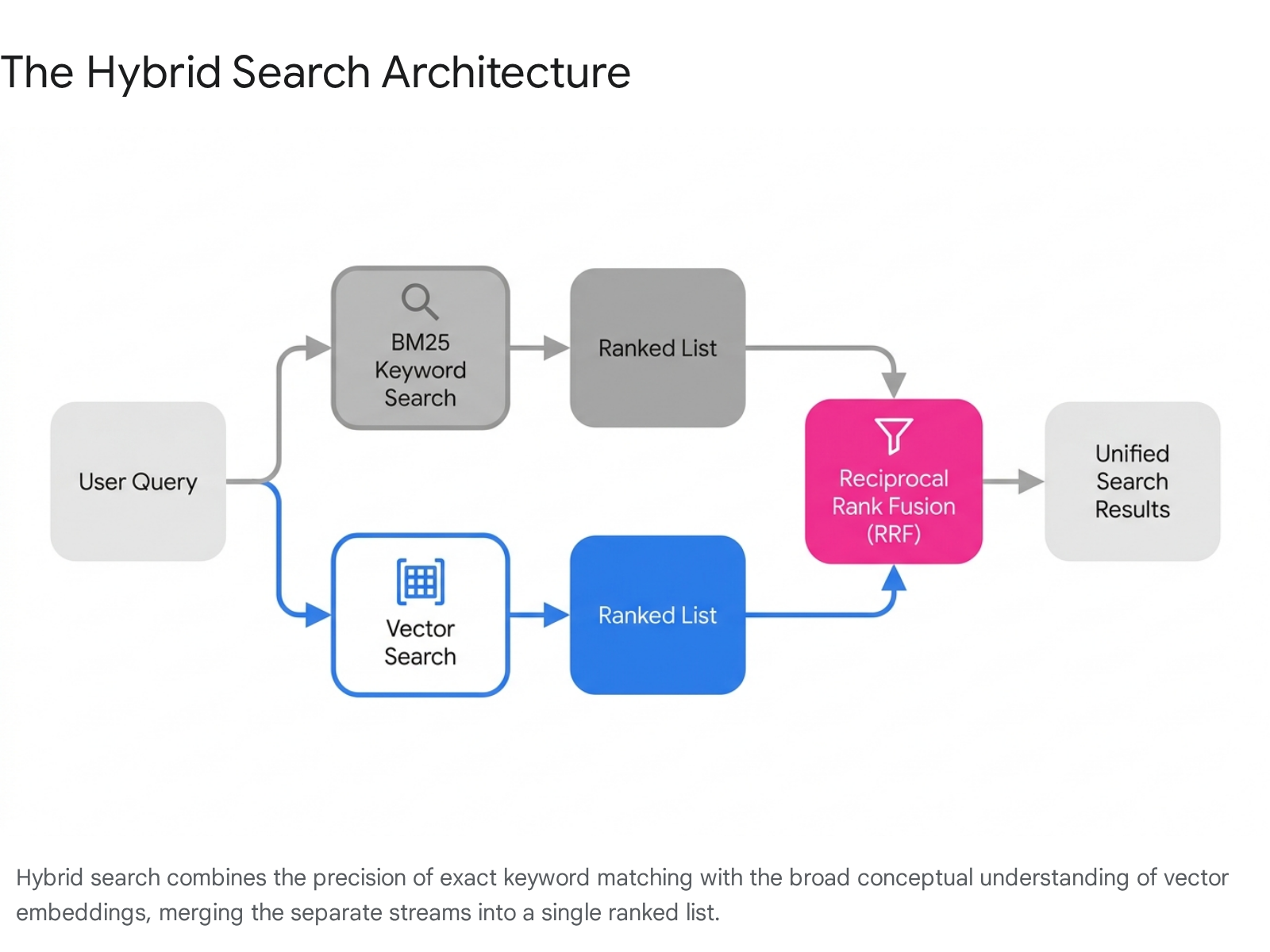
Reciprocal Rank Fusion (RRF)
The primary challenge of hybrid search lies in merging the dual result streams. How does an algorithm reconcile a vector search cosine similarity score of 0.85 with a keyword search BM25 score of 12.4? These figures operate on entirely disjointed mathematical scales 36. Standardizing them through normalization (like min-max or L2) is highly susceptible to extreme outliers, where an anomalous score from one search engine can completely dominate and distort the final ranking 37.
To resolve this seamlessly, databases utilize a "zero-shot" ranking algorithm called Reciprocal Rank Fusion (RRF) 736. Rather than attempting to translate the raw scores into a common metric, RRF abandons the scores entirely and focuses strictly on the rank position of the documents 363738.
The algorithm applies a simple formula to each retrieved document across both lists: 1 / (k + rank), where rank is the position the document achieved in the specific search, and k is a smoothing constant (most commonly set to 60) 333639. The system calculates this value for the document's position in the keyword results, calculates it for the vector results, and adds the fractions together to produce a unified score 3339.
RRF functions as an elegant consensus mechanism. It rewards documents that consistently appear near the top of multiple algorithms. A document ranking #10 on both the keyword and vector lists will achieve a higher combined RRF score than a document ranking #1 on the keyword list but remaining completely undetected by the semantic engine 3637. By prioritizing this intersection of agreement, RRF reliably surfaces topically accurate and contextually meaningful results without requiring complex machine learning model training or hyperparameter tuning 3738.
Powering the Generative AI Boom
The sudden explosion in the popularity of vector databases throughout 2023 and 2024 was largely driven by the maturation of Large Language Models (LLMs) like GPT-4 6162. While LLMs are highly capable, they suffer from two critical flaws: their training data has a strict cutoff date, and they are prone to "hallucinations" - inventing facts when they lack specific knowledge 47. Furthermore, an enterprise cannot easily or cheaply fine-tune a massive foundational model every time an internal policy document is updated 6140.
The solution to this dilemma is an architectural pattern known as Retrieval-Augmented Generation (RAG), with the vector database serving as the critical central nervous system 1364.
When a RAG pipeline is deployed, proprietary enterprise data - such as internal wikis, financial reports, or support logs - is ingested and split into manageable "chunks" of text (typically 300 to 500 tokens) 172241. These chunks are passed through an embedding model and stored permanently in the vector database alongside their metadata 1741.
The operational workflow follows a strict sequence:
1. Query Processing: An employee asks a chatbot a question (e.g., "What is our remote work policy for international contractors?") 4042.
2. Retrieval: The application embeds the user's question into a vector and queries the database 4143. The vector database performs a high-speed ANN similarity search, identifying the top K most semantically relevant text chunks from the proprietary data 4168.
3. Augmentation and Generation: The application retrieves the raw text of these matched chunks and injects them directly into the LLM's context window alongside the original prompt 174741. The LLM reads the retrieved evidence and generates a highly accurate, grounded response that cites its sources, bypassing the need to rely on its internal training weights 224741.
By acting as the high-speed "external memory" for language models, vector databases transform generalized AI into secure, domain-specific enterprise tools 5340.
The Vector Database Ecosystem
As the demand for high-dimensional search has intensified, the database ecosystem has bifurcated into two distinct philosophies: purpose-built infrastructure and extended traditional databases.
Purpose-built vector databases - such as Pinecone, Milvus, Qdrant, and Weaviate - were engineered from the ground up explicitly to handle the unique challenges of embeddings and ANN indexing 51821. Because indexing graph structures like HNSW are highly memory-intensive, these platforms focus heavily on horizontal scalability, distributed cluster management, and advanced features like hybrid search and integrated metadata filtering 532. Pinecone, for example, abstracts infrastructure management entirely via a serverless architecture 3043. Milvus targets massive billion-scale operations by sharding data across distributed nodes, while Qdrant emphasizes performance efficiency utilizing the Rust programming language and payload indexes 2130.
Conversely, established database vendors have adapted to the AI era by building vector capabilities directly into their existing products. PostgreSQL achieved this via the popular pgvector extension, while systems like Elasticsearch, MongoDB, and Redis integrated native vector search features 51221. For organizations already entrenched in these relational or NoSQL ecosystems, these extensions provide a seamless way to add semantic capabilities to existing structured data without adopting entirely new operational pipelines 81221.
Bottom line
Vector databases solve the limitations of literal keyword matching by translating text, images, and audio into high-dimensional numerical coordinates, allowing algorithms to search by semantic intent. To navigate massive datasets at sub-millisecond speeds, these systems employ Approximate Nearest Neighbor (ANN) indexes - like the multi-layered HNSW graph or clustered IVF structures - trading marginal recall accuracy for exponential performance gains. As the foundational memory layer for Retrieval-Augmented Generation (RAG) applications, vector databases have cemented their role in the modern infrastructure stack, with hybrid search and Reciprocal Rank Fusion ensuring systems deliver the perfect blend of conceptual understanding and exact precision.