How to Avoid Overfitting in AI Swing-Trading Models
Avoid overfitting an AI swing-trading model by discarding traditional randomized cross-validation in favor of time-aware methodologies like walk-forward analysis and purged cross-validation. You must rigorously limit your model's parameter count to variables that exhibit broad performance plateaus, and apply mathematical penalties like the Deflated Sharpe Ratio to correct for the inherent optimism of multiple testing. Ultimately, bridging the gap between backtests and live trading requires penalizing historical simulations with realistic execution friction, slippage, and cross-market validation.
The Epistemological Trap of Financial AI
In traditional machine learning applications, such as image recognition or natural language processing, data points are generally independent, and the signal-to-noise ratio is exceptionally high. A picture of a cat today looks structurally identical to a picture of a cat tomorrow. Financial markets, however, operate under entirely different physical laws. They are characterized by a vanishingly low signal-to-noise ratio, continuous non-stationarity, sudden regime switching, and market reflexivity, wherein the act of trading alters the underlying data 12.
When an artificial intelligence model attempts to find patterns in this environment, it is highly susceptible to overfitting. Overfitting occurs when an algorithm learns the training data too perfectly, modeling the random noise, microscopic idiosyncrasies, and specific historical fluctuations of a dataset rather than discovering a genuine, underlying market signal 2345. In plain English, an overfit model memorizes its training data instead of learning a generalizable, predictive rule 46.
If an AI's trading rules are tuned tightly enough to the specific quirks of a historical price series, the strategy will produce an astonishing, flawlessly upward-trending equity curve during backtesting, only to hemorrhage capital the moment it is deployed in live markets 4578. The AI has essentially become an expert historian rather than a reliable forecaster.
High Dimensionality and Low Sample Counts
Financial time series frequently present a structural paradox known to data scientists as a "high dimensionality, low sample count" environment 2. A swing trader might feed their model hundreds of distinct variables: open, high, low, and close price movements, trading volumes, complex technical indicators, macroeconomic interest rate data, and even alternative data streams like social media sentiment 26.
Yet, on a daily timeframe, there are only about 252 trading days in a calendar year. When an algorithm possesses thousands of parameters and a relatively small number of independent market events to learn from, it is granted far too many degrees of freedom 29. Given infinite computational power and a finite dataset, an AI will inevitably find a mathematical formula that perfectly predicts the past by pure statistical coincidence 27.
The Illusion of the Perfect Equity Curve
The reason overfitting is so deeply seductive in quantitative finance is that the same historical data window often serves as both the playground for discovery and the ultimate scoreboard for validation 4. You build a strategy on the same historical prices you use to grade its efficacy. Every incremental improvement you make to the algorithmic rules is implicitly informed by the data you are testing against. You are not discovering an edge; you are merely describing what already happened 4.
The honest test of a financial model - and arguably the only one that truly matters - is whether the strategy generates consistent profitability on entirely unseen data that the system was quarantined from during development 46.
Flaws in Traditional Validation Methods
In standard data science, the gold standard technique for preventing overfitting is K-fold cross-validation 10. The dataset is randomly shuffled and divided into an arbitrary number of equally sized chunks, or "folds." The model is repeatedly trained on most of the folds while being evaluated on a hold-out test fold, and the results are averaged to provide a stable estimate of performance 101.
When applied to sequential financial time series, however, standard K-fold cross-validation is often disastrous. Shuffling the dataset completely destroys all temporal dependencies, creating an environment where the validation set frequently occurs chronologically before the training set 1012.
Look-Ahead Bias and Data Leakage
By evaluating a model out of chronological order, standard cross-validation trains the AI on future market data to predict past market events 1012. This is a textbook case of data leakage, commonly referred to in quantitative finance as look-ahead bias 102. In live trading, you never have access to future volatility regimes, sudden price shocks, or macroeconomic shifts. Naive cross-validation collapses into a flawed simulation that grants the model false comfort by leaking future structural changes into the training set 10122.
Even simple chronological train-test splits, where a researcher trains on the first 80% of data and tests on the final 20%, carry risks. While this prevents look-ahead bias, it implicitly biases the model toward the most recent market regime and leaves a massive portion of historical data unused for validation 17.
Evaluating Validation Methodologies
To accurately gauge how an AI model will perform in the real world, quantitative researchers must respect the causal, sequential arrow of time. The table below summarizes the core differences between validation methods in algorithmic trading.
| Validation Methodology | Core Mechanism | Primary Flaw in Financial Modeling | Best Practical Use Case |
|---|---|---|---|
| Standard Train-Test Split | Splits data sequentially into two blocks (e.g., train on 2015-2020, test on 2021-2023). | Biases the model toward the most recent market regime and leaves older data untested 1. | Quick baseline evaluations and early-stage hypothesis testing 17. |
| Standard K-Fold Cross-Validation | Randomly shuffles and partitions data into K folds for iterative testing. | Causes catastrophic data leakage by training on future events to predict past events 10122. | Cross-sectional datasets predicting static fundamentals, rarely used for time series 12. |
| Walk-Forward Analysis (WFA) | Trains on a historical block, tests on the immediate future block, then "rolls forward" chronologically 11014. | Computationally expensive; older market regimes receive less out-of-sample testing validation 115. | Live trading simulations for strategies sensitive to shifting macroeconomic regimes 14. |
| Purged and Embargoed K-Fold CV | Partitions data sequentially, mathematically removing overlapping data between train and test sets 216. | Requires highly advanced coding frameworks and careful management of fractional differentiation 1217. | Complex machine learning and AI models requiring maximum data efficiency without leakage 1216. |
Advanced Time-Aware Validation Frameworks
To resolve the inadequacies of standard techniques, the quantitative finance community has developed highly robust, time-aware validation frameworks designed to punish overfit models before they ever reach live execution.
Walk-Forward Optimization
Walk-forward optimization is widely considered the most intuitive and effective approach for algorithmic swing traders. It is designed specifically to simulate real-world deployment by respecting the strict chronological order of the data 110.
Instead of evaluating the strategy on one massive block of out-of-sample data, the process is iterative. You train your AI on a specific historical window (for example, three years of data), test it on the immediate, unseen subsequent block (e.g., the following six months), and then shift the entire training window forward in time 11014. This rolling scheme is repeated until the present day is reached.
This method continually forces the model to adapt to new information, providing a highly realistic view of how the model would have survived shifting market environments 114. It answers the critical question: if you had deployed this model live five years ago, retraining it periodically as new data arrived, what would your actual equity curve look like today?
Combinatorial Purged Cross-Validation (CPCV)
For more complex AI models that require maximum data retention to learn structural patterns, financial machine learning expert Marcos López de Prado introduced the concept of Purged and Embargoed K-Fold Cross-Validation 12216.
Financial events frequently overlap in time. If an AI swing trade is designed to last ten days, a data point recorded on day four inherently contains embedded, forward-looking information about the eventual outcome on day ten. If you slice a dataset blindly, your training set might contain the data from day ten, while your test set evaluates day four. The AI will inadvertently "learn" the future 122.
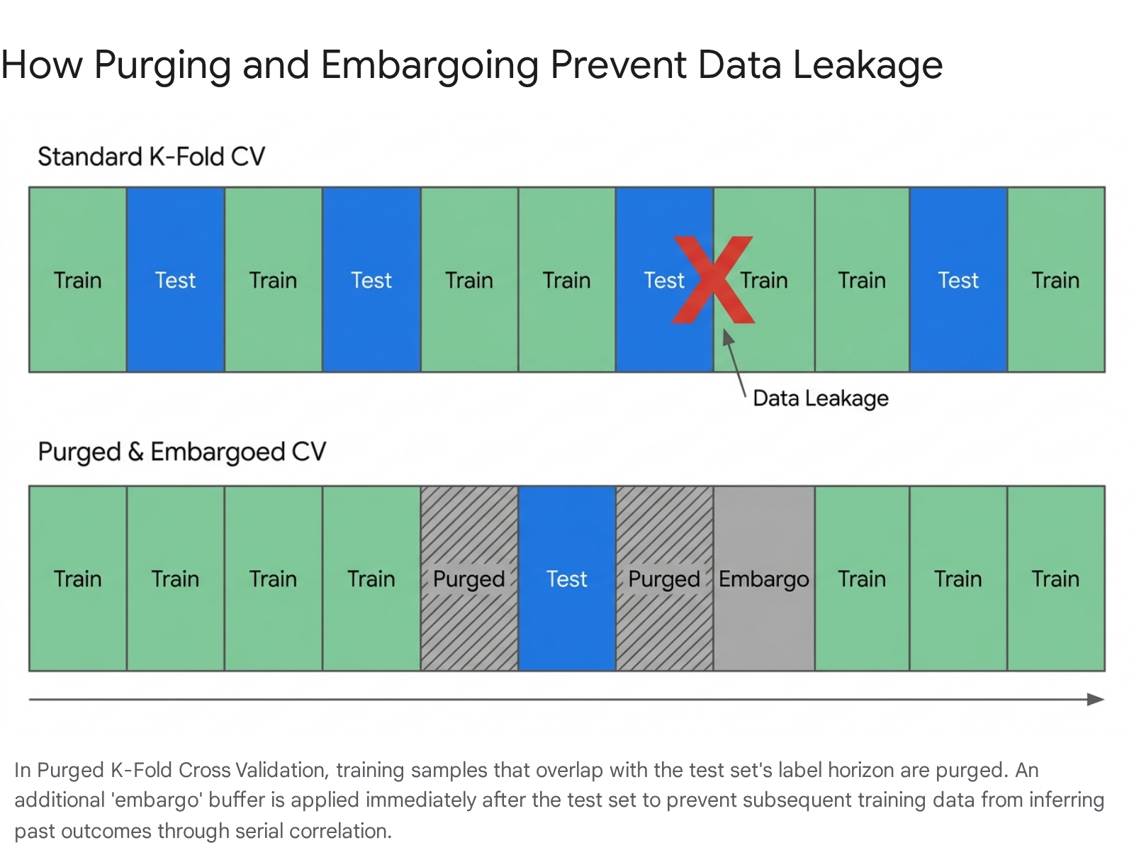
Purged and Embargoed validation solves this through two distinct mathematical mechanisms: * Purging: This step mathematically removes any training observations whose evaluation timeframes overlap in any capacity with the testing set horizon 12217. This ensures the training data remains entirely "future-free." * Embargoing: Financial markets exhibit intense serial correlation, meaning prices today heavily influence prices tomorrow. Embargoing drops an additional block of training data immediately after the test period. This acts as a quarantine buffer, ensuring the model cannot indirectly infer the test set's results from the immediate market aftermath 1221617.
By enforcing strict temporal isolation, Purged K-Fold validation allows developers to utilize more of their historical data for deep learning without the fatal risk of look-ahead bias 12.
Strategies for Model Architecture and Parameter Limits
A fundamental law of quantitative trading dictates that the complexity of an algorithmic model must be deeply justified by the complexity of the actionable signal. Over-engineering is the enemy of robustness.
The Plateau Test versus Razor-Thin Peaks
Retail traders and inexperienced institutional analysts frequently fall into the trap of grid optimization. This involves utilizing vast computational power to test thousands of minor variations of a strategy - such as adjusting a moving average from 40 days, to 41 days, to 42 days - until they find the one hyper-specific setting that maximizes the backtest's performance metrics 141819.
This practice invariably leads to a model that is fragile and dangerously tailored to a specific historical dataset. A practical rule of thumb is to strictly limit your explicit parameters (the inputs directly manipulated by the trader or the algorithm) to a bare minimum, often between two and five key variables 1420.
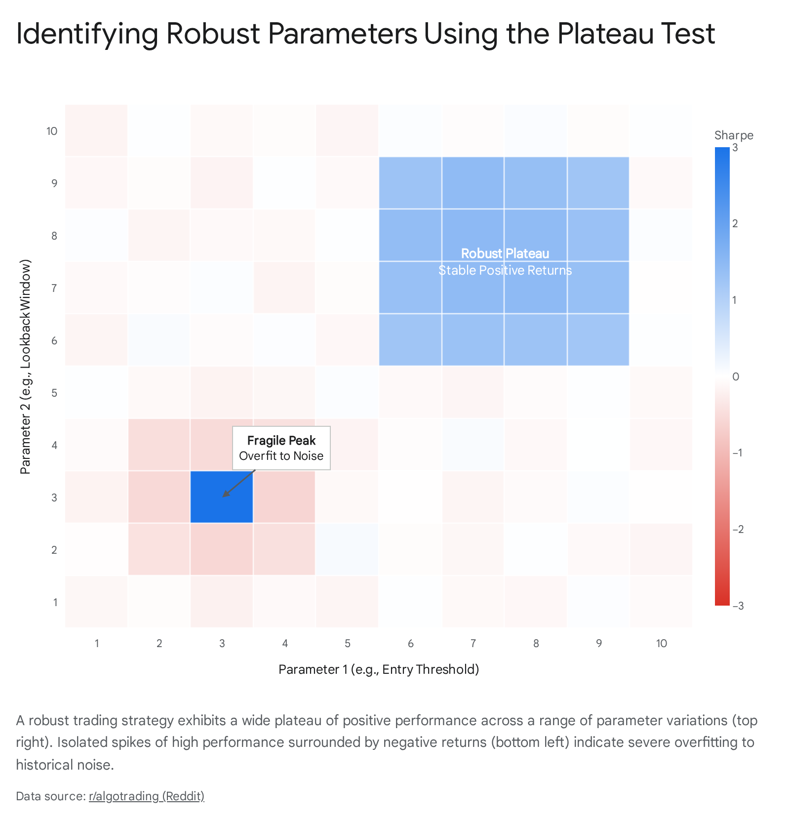
More importantly, the algorithm must pass the "plateau test" 18. If you plot your AI's historical performance across a wide spectrum of different parameter settings, you must look for broad, stable plateaus of profitability. If your model requires an exact 14-period lookback window to be profitable, but begins losing money rapidly at 13 periods and 15 periods, the edge is a statistical illusion - a razor-thin peak built on noise 18.
If perturbing any parameter by 15% in any direction causes the strategy's risk-adjusted returns to plummet by more than 25%, the strategy is severely overfit, regardless of how few parameters it employs 18. Robustness lives in the broad geometry of the optimization surface, not in a single perfect configuration 18.
Transformers vs. Traditional Machine Learning
When selecting the architecture for an AI swing-trading model, quantitative developers frequently debate the merits of massive deep learning models against traditional, simpler machine learning frameworks.
Recent research into Transformers - the architecture underpinning generative Large Language Models - shows profound potential in forecasting financial time series 21345. Unlike Long Short-Term Memory (LSTM) networks or Recurrent Neural Networks (RNNs) that process data sequentially step-by-step, Transformers utilize a "self-attention" mechanism to process entire data sequences simultaneously 21525. This allows the architecture to effectively weigh the importance of distant historical events against recent market volatility, distinguishing between temporary market noise and genuine structural trend changes 21326. In high-noise environments where traditional filtering methods like moving averages or Kalman filters collapse, time-aware Transformers have demonstrated a unique ability to maintain low error rates 2125.
However, increased capacity brings an exponentially increased risk of overfitting. Deep neural networks, with their vast parameter counts, are incredibly efficient at memorizing noise 3527. In numerous empirical studies evaluating daily stock returns, traditional models like Autoregressive Integrated Moving Average (ARIMA) or Random Forests remain incredibly difficult to beat when datasets are limited or characterized by high idiosyncratic noise 629. Furthermore, while Transformers excel at predicting absolute price sequences and long-term dependencies, specialized LSTM models often demonstrate superior and more consistent performance in predicting short-term differential sequences, such as minute-by-minute price movements 478.
Applying Regularization and Denoising
If you elect to employ a high-capacity Transformer or LSTM, you must utilize aggressive regularization techniques to prevent the model from memorizing the training data. Implementing moderate dropout rates (between 0.18 and 0.23), early stopping protocols, and careful feature selection are mandatory practices 625.
Additionally, because financial data is highly erratic, integrating an autoencoder into the architecture to denoise the data before it reaches the predictive layers can force the model to learn only the most dominant, persistent features, significantly reducing the likelihood of curve-fitting 2632.
Statistical Tools to Quantify and Penalize Overfitting
Perhaps the most insidious form of overfitting occurs before the AI even finishes its final training run. It is an epistemological blind spot known to statisticians as the multiple testing problem 3334.
If you design a purely random strategy, test it once, and discard it, you have successfully avoided a bad model. But if you systematically generate and test thousands of random strategy variations using AI, basic probability dictates that several of them will produce extraordinary, statistically significant backtests entirely by chance 3435. Because modern quants can test in twenty minutes what used to take a research team a month, the survivorship bias in algorithmic research is brutal 436. The strategy you finally select isn't necessarily the smartest or most predictive; it is simply the one that randomly mapped perfectly onto historical noise 434.
To combat this illusion, researchers rely on a suite of advanced statistical metrics designed to penalize overly aggressive backtesting.
The Probability of Backtest Overfitting (PBO)
Developed by David H. Bailey, Marcos López de Prado, and colleagues, the Probability of Backtest Overfitting (PBO) measures the overarching risk of your research pipeline 33938.
PBO is calculated using a technique called Combinatorially Symmetric Cross-Validation (CSCV). This method groups the performance metrics of thousands of strategy trials into submatrices 394010. It systematically tests whether the specific parameter combinations that perform optimally in-sample routinely collapse out-of-sample across different combinations of the dataset 4010.
A high PBO indicates that your research process itself is compromised. It flags that the strategies appearing "best" in your training environment are highly likely to underperform the median strategy in unseen environments, proving that your success is the product of random variance rather than a persistent structural edge 333810.
The Deflated Sharpe Ratio (DSR)
A backtest Sharpe ratio of 2.0 sounds impressive to investors, but it is statistically meaningless without proper context 344243. The Deflated Sharpe Ratio (DSR) corrects the standard Sharpe ratio by mathematically penalizing it based on the realities of your research and data-mining process 111213.
The standard Sharpe ratio naively assumes a normal distribution of returns and ignores the number of attempts it took to find the strategy. The DSR actively discounts your performance metric by factoring in five critical variables: 1. The number of independent trials tested: The more backtests you ran to discover the strategy, the heavier the mathematical penalty applied to your final score. Trying harder does not equal genuine skill 4311. 2. The variance of the trials: If the performance of your discarded strategies varied wildly, the penalty increases 1113. 3. Sample length: Shorter backtests are penalized far more heavily than multi-year simulations 3413. 4. Non-normality of returns (Skewness and Kurtosis): Standard Sharpe estimates misinterpret higher moments. If your AI's returns exhibit negative skewness or excess kurtosis - meaning it relies on frequent small wins masking occasional, catastrophic losses - the DSR severely deflates the apparent skill 1213.
False Discovery Rate (FDR)
While PBO measures the fragility of your overall research process, the False Discovery Rate (FDR) acts as a complementary metric to control the proportion of false positives 3314. When you test multiple strategy configurations, some will pass traditional significance thresholds purely by luck. FDR provides a conservative estimate, answering the question: out of the strategies that appear profitable, what percentage are likely false discoveries? Monitoring FDR forces algorithmic traders to maintain a healthy skepticism of their own backtesting pipelines, recognizing that a high passing rate is often a red flag for widespread data leakage 33.
Bridging the Execution Gap: Backtest vs. Live Reality
The final hurdle in avoiding algorithmic overfitting is ensuring your AI model survives the brutal transition from the sterile, frictionless laboratory of a historical backtest into the chaotic reality of live financial markets. It is an industry standard among quantitative professionals to expect a 20% to 50% performance decay between a highly optimized backtest and live trading execution 154950. Short-term and high-frequency strategies typically experience the most severe drops 49.
Modeling Transaction Costs and Market Impact
Backtests routinely lie by omission. They often naively assume that limit orders are executed the precise millisecond a price is touched, ignoring order book queue position and partial fills 4950. Furthermore, AI models tested on clean, end-of-day datasets are entirely blind to intraday volatility, widening bid-ask spreads during market shocks, and the millisecond latency that relentlessly erodes live profits 849.
To prevent your AI from overfitting to a frictionless fantasy, your backtest engine must strictly enforce real-world constraints. This includes aggressive transaction costs, realistic slippage penalties based on available market volume, and explicit borrow fees for any short positions, which can often range from 1% to 10% annually and transform profitable short theses into outright losses 9192750.
Point-in-Time Data and Survivorship Bias
The quality of your historical data is paramount; garbage in guarantees garbage out 8. A massive source of overfitting is the accidental use of restated financial data. If your model evaluates corporate earnings or book value using today's cleaned database values for historical periods, you are granting the AI look-ahead bias, as those restated numbers were not available to traders at the actual time of the event. Utilizing a strictly point-in-time database is mandatory 9.
Similarly, testing a strategy exclusively on the current constituents of an index like the S&P 500 introduces massive survivorship bias. The AI implicitly "knows" that all companies in the current dataset eventually survived and succeeded, ignoring the hundreds of companies that were historically delisted due to bankruptcy 8361652. A model that inadvertently learns to buy failing companies will appear miraculously profitable in a survivorship-biased backtest because those companies simply vanish from the record, but the strategy will accumulate devastating losses in live trading 36.
Cross-Market Validation and Geographical Robustness
A powerful and definitive test of an AI model's robustness is out-of-sample cross-market validation 53. If your AI model identifies a seemingly brilliant swing-trading edge in U.S. equities, you should deploy the exact same architecture, without altering its hyperparameters, onto entirely unrelated markets, such as the Chinese SSE50 or the Indian Nifty50 54.
If the model relies on universal behavioral anomalies - such as human overreaction to geopolitical news, microstructure liquidity gaps, or structural mean-reversion - it should demonstrate at least marginal, consistent profitability across different geographies 5355. Conversely, if the system completely implodes outside of the U.S. technology sector, it strongly indicates that the AI has overfit to local, temporary market dynamics rather than discovering a fundamental, transferable law of trading 5354.
Bottom line
To avoid overfitting an AI swing-trading model, developers must abandon standard randomized cross-validation and implement strictly chronological, purged, and embargoed data splits that prevent future information leakage. Algorithmic complexity must be constrained by rigorous parameter limits and the plateau test, while historical performance must be evaluated using the Deflated Sharpe Ratio to mathematically discount the illusion of success generated by testing thousands of variations. Ultimately, no historical simulation can capture the full friction of live execution; sustained success requires recognizing that backtests are tools for disproving fragile ideas, not guarantees of future wealth.