
Using Technical Indicators as Machine Learning Features
BLUF The transition from discretionary trading to machine learning-driven algorithmic trading requires a fundamental shift in how market data is processed and interpreted. Retail developers frequently fail because they feed non-stationary raw prices and unscaled, highly correlated technical indicators directly into off-the-shelf predictive models - falling victim to the "raw price" and "kitchen sink" misconceptions. Building a robust financial machine learning model necessitates transforming price histories into memory-preserving stationary features via fractional differentiation, contextualizing bounded and unbounded indicators through rigorous mathematical scaling, and preventing look-ahead bias through purged and embargoed cross-validation. While advanced deep learning architectures like the Momentum Transformer show promise in handling specific sequence modeling tasks, highly optimized tree-based models like XGBoost trained on meticulously engineered tabular features consistently offer superior performance, stability, and interpretability in noisy financial markets.
The Allure of AI Trading: A Modern Mirage?
Consider the scenario of a contemporary retail trader in the year 2026. Armed with a laptop, access to zero-commission brokerage APIs, and an array of large language models capable of generating Python scripts in seconds, the technical barrier to entry for algorithmic trading has been completely obliterated 12. The internet is saturated with tutorials promising that an amateur can spin up an artificial intelligence trading bot in thirty minutes, backtest it over five years of historical equity or cryptocurrency data, and deploy it to generate automated, emotionless returns 2. The global algorithmic trading market is projected to grow to over $28 billion by 2030, with retail investors now accounting for approximately 43% of the market participation 234.
However, a sweeping longitudinal study - the largest of its kind, covering 28 years of continuous trading data across 8 million retail profiles and 295 million trades - reveals a profoundly sobering reality. Between 74% and 89% of retail traders lose money, a failure rate that has remained remarkably static across the dot-com bubble, the 2008 financial crisis, the COVID-19 boom, and multiple cryptocurrency cycles 517. Regulatory bodies corroborate these findings; the European Securities and Markets Authority (ESMA) and the US Commodity Futures Trading Commission (CFTC) consistently report that over 70% of retail foreign exchange and Contract for Difference (CFD) traders sit in the red, with some 2024 averages indicating that 86% of retail forex traders lose capital 5. A 2025 survey of retail cryptocurrency traders found that 84% lost money in their first year, with 58% losing nearly all their starting capital due to poor research and behavioral biases 5.
These staggering losses are rarely due to a lack of computational power or access to information. Instead, they stem from structural, behavioral, and data-hygiene errors 58. Hobbyists often assume that machine learning models possess an intrinsic, human-like understanding of the financial markets. They build bots that memorize the past rather than learn generalizable strategies, they ignore market microstructure and transaction costs, and most fatally, they fundamentally misunderstand how to engineer data so that an algorithm can accurately interpret it 19. As institutions invest heavily in low-latency infrastructure, advanced quantitative research, and complex regulatory compliance frameworks under MiFID II, the disparity between institutional rigor and retail plug-and-play models has never been wider 34102.
Why Do Most Retail AI Trading Bots Fail?
The failure of retail algorithmic trading is frequently misattributed to a lack of emotional discipline, but empirical data indicates the issue is deeply structural and mathematical 8. When non-institutional developers attempt to apply machine learning to financial markets, they typically fall into several well-documented traps, primarily driven by two massive misconceptions regarding feature engineering.
The first critical error is the "Kitchen Sink" misconception. Because technical indicators are easy to calculate using open-source libraries, amateur developers often generate dozens of indicators - Simple Moving Averages (SMA), Exponential Moving Averages (EMA), Relative Strength Index (RSI), Moving Average Convergence Divergence (MACD), Bollinger Bands, and Stochastic Oscillators - and feed all of them into a predictive model simultaneously 12131415. The underlying assumption is that the machine learning algorithm will automatically sort out which indicators are important and discard the rest.
In reality, many technical indicators are mathematically collinear; they are direct derivations of the exact same underlying price and volume data 3. Feeding a model an RSI, a Stochastic Oscillator, and a Commodity Channel Index (CCI) provides redundant momentum signals that measure the same underlying phenomenon 12. In high-dimensional spaces, this multicollinearity causes weak but genuine predictive signals to be drowned out by the sheer volume of irrelevant noise 9. This redundancy confuses gradient descent algorithms, destabilizes feature importance metrics in tree-based models, and leads directly to overfitting 13. The model learns the exact noise of the training data but fails catastrophically in live, out-of-sample trading 1. Successful quantitative models do not rely on stacking redundant indicators; they rely on selecting orthogonal features that capture distinct dimensions of market behavior, such as momentum, volatility, and mean reversion 133.
The second fatal error is the "Raw Price" misconception. Countless tutorials demonstrate training deep neural networks by feeding them raw closing prices 17. This is a fundamental violation of statistical modeling principles. Machine learning algorithms, particularly those used in supervised learning, operate under the strict mathematical assumption that the data is stationary - meaning its statistical properties, such as its mean, variance, and autocorrelation, remain constant over time 184205. Raw asset prices are inherently non-stationary; they drift, trend, and undergo violent regime changes driven by macroeconomic factors 174. A model trained to recognize that a stock is a "strong buy" at $150 will experience catastrophic failure when the stock splits, or when inflation drives the baseline price to $300. Feeding non-stationary raw prices to a model ensures that the algorithm will break as soon as the market breaches its historical price boundaries 17420.
Why Can't Raw Price Data Be Fed Directly into a Predictive Model?
To understand why raw prices destroy predictive models, one must understand the delicate, often contradictory balance between stationarity and memory in financial time series analysis.
As established, covariance stationarity is the bedrock requirement for robust statistical modeling, ensuring that the mean and variance of different data partitions remain consistent over time 18420. To achieve this stationarity, the conventional wisdom in quantitative finance has been to transform raw prices into fractional or logarithmic returns 22. By subtracting yesterday's price from today's price, the data is differenced at an integer order of 1. This mathematical operation successfully removes the long-term trend and creates a stationary series that oscillates around a constant mean, typically near zero 2223.
However, there is a severe analytical cost to integer differentiation: it completely obliterates the "memory" of the time series 5226.
To grasp this concept, consider an analogy based on the mathematics of cooking, scaling, and fraction manipulation. Imagine following a complex recipe to bake a pie 25. During the preparation phase, you can manipulate the raw ingredients using simple fractional scaling 2627. If you want to make a larger pie, you can multiply the $\frac{1}{2}$ cup of sugar, the $\frac{3}{4}$ cup of milk, and the 2 cups of flour by $1\frac{1}{2}$ 262728. Because the ingredients are still separate and raw, their intrinsic properties are preserved, and their relationships scale perfectly 2628. You retain complete control over the individual components 25.
However, once you combine the ingredients and subject them to the extreme, transformative heat of an oven, a non-reversible chemical reaction occurs 2529. You cannot take a fully baked pie and reverse-engineer it to extract the original raw eggs or the flour 25. The ingredients have interacted in complex, simultaneous ways that destroy their isolated states 25.
In quantitative finance, integer differentiation is the equivalent of baking the pie. When a developer calculates a daily return, they are mathematically discarding every single piece of price history that occurred prior to the previous day 2223. The resulting time series of returns is stationary, but it is entirely memory-less 22. The machine learning model sees that the asset increased by 2% today, but it has absolutely no memory of whether the asset has been in a massive, compounding bull run for the last five years, or if it is merely experiencing a dead-cat bounce during a decade-long bear market. Applying complex machine learning algorithms to these memory-erased series forces the model to hunt for patterns in isolated data points, frequently leading to false discoveries and entirely eroding the model's predictive power 2230.
What Is Fractional Differentiation and Why Does It Matter?
To resolve the paralyzing dilemma between memory-rich non-stationary prices and memory-less stationary returns, Dr. Marcos Lopez de Prado pioneered the application of fractional differentiation to financial machine learning 522.
Fractional differentiation rejects the binary choice of leaving data raw (an integer differentiation order of 0) or completely converting it to returns (an integer differentiation order of 1) 2231. Instead, it allows the degree of differencing - denoted as $d$ - to be a real, fractional number between 0 and 1 631. The objective is to engineer a "Golden Mean": discovering the minimum amount of differentiation required to achieve stationarity while actively preserving the maximum amount of historical memory 522.
Mathematically, this is achieved by expanding the backshift operator using an infinite binomial series 236. Unlike integer differentiation, where the weight of yesterday's price is -1 and all previous prices drop abruptly to 0, fractional differentiation applies a sequence of weights to past prices that decay non-linearly over time 236. The weights alternate in sign and slowly converge toward zero, ensuring that older price points still exert a mathematically precise, albeit diminishing, influence on the current observation 630.
In practice, a quantitative researcher will iteratively apply increasing fractional values of $d$ to a price series and subject each resulting series to an Augmented Dickey-Fuller (ADF) test 52330. The ADF test checks for the presence of a unit root; if the p-value falls below a critical threshold (typically 0.05, representing a 95% confidence level), the null hypothesis of non-stationarity is rejected 1822. If a time series requires a $d$ value of 0.4 to pass the ADF test, the researcher applies exactly 0.4 differentiation 2330. This acts as a specialized, memory-preserving filter 307. The resulting time series is mathematically proven to be stationary - satisfying the strict requirements of supervised machine learning algorithms - yet it retains the long-term historical dependencies and trends that give a predictive model its statistical edge 307.
How Are Technical Indicators Translated into Machine Learning Features?
Technical indicators are effectively the "cockpit instruments" of algorithmic trading, transforming raw Open, High, Low, Close, and Volume (OHLCV) data into mathematical representations of momentum, trend, and volatility 1233. However, translating these indicators into machine-learning-ready features requires careful contextualization.
A machine learning algorithm does not inherently understand that a Relative Strength Index (RSI) reading of 30 implies an "oversold" market condition. It simply processes the integer 30. If indicators are not properly bounded, scaled, and engineered, the model will fail to interpret their significance across different market regimes 13. The goal is to provide the algorithm with context.
Relative Strength Index (RSI)
The RSI, developed by J. Welles Wilder, is a momentum oscillator that measures the speed and magnitude of recent price changes to evaluate whether an asset is overbought or oversold 123334. It is calculated by dividing the exponentially smoothed average of gains by the average of losses over a specified lookback window, typically 14 periods 133536. The RSI is highly suitable for machine learning because it is naturally bounded between 0 and 100 123337. Because it is strictly bounded and calculated as a relative ratio independent of the absolute asset price, it typically exhibits stationary properties and can be fed into machine learning algorithms with minimal preprocessing 37. However, rather than just feeding the raw RSI value, sophisticated feature engineering captures RSI Divergence 1238. By creating a feature that calculates the difference between the slope of the price trend and the slope of the RSI over a rolling window, the model is explicitly taught to recognize fading momentum 1238. A positive price slope converging with a negative RSI slope provides a powerful, pre-calculated reversal signal that the model does not have to learn from scratch 1238.
Moving Average Convergence Divergence (MACD)
The MACD is a trend-following momentum indicator calculated by subtracting a slow Exponential Moving Average (EMA), typically 26 periods, from a fast EMA, typically 12 periods 141539. A 9-period EMA of the resulting MACD line is then plotted alongside it as a "signal line," with the difference between the two represented as a histogram 36398. Unlike the RSI, the raw MACD is wildly unbounded and heavily dependent on the absolute price of the underlying asset 37. A raw MACD value of 5.0 is completely meaningless without context; it could represent a massive momentum shift on a $10 stock, or microscopic, irrelevant noise on a $3,000 index 37. Therefore, raw MACD values must never be fed directly into a machine learning model 37. To make the MACD stationary and cross-asset comparable, it must be normalized 3739. One standard method is to divide the MACD value by the absolute underlying price, transforming it into a Percentage Price Oscillator (PPO) 3739. Advanced institutional scaling methods involve normalizing the MACD relative to its own signal line using formulas such as $r_{MACD} = \frac{MACD_t - SIG_t}{0.5(|MACD_t| + |SIG_t|)}$, which bounds the feature strictly between -1 and 1 while preserving the magnitude of the divergence 35.
Bollinger Bands
Bollinger Bands are a primary volatility indicator consisting of a middle band (usually a 20-day Simple Moving Average) and upper and lower bands set a specified number of standard deviations (usually two) away from the middle band 333641. As volatility increases, the bands expand; as it decreases, they contract 33. Because the absolute values of the bands are simply price levels, they are inherently non-stationary and useless to a predictive model. Feature engineering requires transforming the bands into relational metrics. The first is "%B" (Percent B), which quantifies exactly where the current price sits relative to the bands: $\%B = \frac{Price - Lower Band}{Upper Band - Lower Band}$. A %B value of 1.0 means the price is touching the upper band, while 0.0 means it is touching the lower band, creating a normalized momentum oscillator 1213. The second necessary feature is "Bandwidth" ($\frac{Upper - Lower}{Middle}$), which explicitly feeds the model a measure of volatility compression. This allows the model to identify "Bollinger Squeezes," where low bandwidth historically precedes explosive directional breakouts 1213.
Average True Range (ATR) & Volume Metrics
The ATR measures absolute market volatility by decomposing the entire range of an asset price for a given period, accounting for gaps between trading sessions 4243. Because it is expressed as an absolute dollar value, it suffers from the same non-stationarity issues as the MACD. Converting ATR into a percentage of the closing price ($\frac{ATR}{Close}$) creates a normalized, stationary feature that accurately models volatility regimes across assets of vastly different prices, allowing algorithms to dynamically adjust position sizing parameters 4243.
Similarly, raw trading volume is notoriously non-stationary and highly prone to extreme outliers caused by earnings reports or macroeconomic announcements 36. Feeding raw volume to a distance-based model will violently skew the calculations. The institutional standard is to use a rolling volume ratio: dividing today's volume by a 20-day or 50-day rolling average of volume 36. This transforms the feature into a stationary metric where a value of 2.0 clearly and consistently indicates "double the normal volume," giving the model a normalized measure of market conviction 36.
Feature Transformation Reference Table
To systematically structure these tools for data science applications, the following table summarizes how standard indicators must be engineered before ingestion by a machine learning model to ensure stationarity and boundedness.
| Indicator | Primary Market Purpose | Raw Boundedness | Stationarity Risk | Recommended ML Feature Transformation |
|---|---|---|---|---|
| RSI (14) | Momentum & Reversion | Bounded (0-100) | Low | Use raw value; Calculate rolling slope to engineer divergence features. |
| MACD (12, 26, 9) | Trend Direction & Strength | Unbounded | High | Normalize via MACD/Price ratio (PPO) or MACD-to-Signal Z-score. |
| Bollinger Bands (20, 2) | Volatility & Squeeze Detection | Unbounded | High | Convert to %B (relative position) and Bandwidth (volatility compression). |
| ATR (14) | Volatility & Risk Sizing | Unbounded | High | Convert to ATR % (ATR divided by Close Price) for cross-asset parity. |
| Volume | Liquidity & Market Conviction | Unbounded | High | Convert to Volume Ratio (Current Volume / 20-Day Rolling Mean Volume). |
| Moving Averages (SMA/EMA) | Trend Filtering | Unbounded | High | Convert to relative distance from price (e.g., $\frac{Close - SMA}{SMA}$). |
What Is Feature Scaling, and Why Does It Matter for Distance-Based Algorithms?
Even after transforming technical indicators into stationary ratios and percentages, their absolute numerical ranges can vary drastically across a dataset. The RSI ranges from 0 to 100, a Volume Ratio might range from 0.5 to 5.0, and a fractionally differenced return might hover around 0.002 4445.
To understand why this is problematic, consider an everyday analogy: comparing human height and weight to assess physical similarity 454647. If a dataset measures height in centimeters (e.g., 180 cm) and weight in kilograms (e.g., 75 kg), a machine learning algorithm does not understand the physical units; it only perceives the raw mathematical magnitude of the numbers 4647. Algorithms that rely on measuring the mathematical distance between data points - such as K-Nearest Neighbors (KNN), Support Vector Machines (SVM), and K-Means Clustering - utilize formulas like Euclidean distance 464748. In this distance calculation, the variance in height (measured in the hundreds) will completely overwhelm the variance in weight (measured in the tens). The model will effectively ignore the weight data simply because the numerical values are smaller, leading to biased and inaccurate clustering 4647.
Feature scaling levels the playing field, ensuring that all features contribute proportionately to the model's loss function without artificial bias toward larger numbers 474950.
The choice of scaling technique is critical and depends heavily on the distribution of the financial data: 1. Standardization (Z-Score Normalization): This technique rescales data so that it has a mean of 0 and a standard deviation of 1 ($z = \frac{x - \mu}{\sigma}$) 495152. This is the most common scaling method for financial data that is approximately normally distributed. It aligns features to a standard bell curve and handles minor outliers well, making it ideal for gradient descent optimization 4548. 2. Min-Max Normalization: This method scales all values to a fixed, bounded range, typically strictly between 0 and 1 ($x' = \frac{x - min}{max - min}$) 455152. While highly useful for specific neural network architectures that require bounded inputs (such as image processing), Min-Max scaling is highly vulnerable to financial outliers. A single flash-crash or unprecedented volatility event can permanently squash the rest of the historical dataset into a microscopic, indistinguishable range 45485052. 3. Robust Scaling: Financial data is notoriously characterized by "fat tails" - extreme, unpredictable outlier events that defy normal distribution 454950. Robust scaling addresses this by using the median and the interquartile range (IQR) instead of the mean and standard deviation 4549. Because the median is insensitive to massive outliers, robust scaling prevents a single black-swan market event from distorting the scale of the entire historical dataset, making it a preferred choice for highly volatile assets like cryptocurrencies 454950.
It is crucial to note that tree-based models, such as Random Forests and XGBoost, operate by finding optimal split points in individual features rather than calculating spatial distances between them 4549. Therefore, tree-based models are largely insensitive to feature scaling 49. However, deep learning models (Neural Networks, LSTMs, Transformers) rely heavily on gradient descent to update their internal weights. If features are unscaled, the neural network's weights will update unevenly, causing the optimization algorithm to oscillate wildly, drastically slowing down training time, and often failing to converge on an optimal solution 44464950. Furthermore, to prevent data leakage, scalers must always be fitted exclusively on the training data, and then used to transform the validation and test sets; fitting a scaler on the entire dataset incorporates future data into the historical scale, compromising the model's integrity 37495052.
How Do I Prevent My Model from Cheating with Look-Ahead Bias?
The single most common reason a retail algorithmic trading model shows 400% returns in historical backtesting but rapidly hemorrhages capital in live trading is data leakage, specifically look-ahead bias 15354.
In standard machine learning classification tasks, data scientists utilize K-Fold Cross-Validation. The dataset is randomly shuffled and split into subsets (folds) to train and test the model repeatedly, ensuring it generalizes well to unseen data 549. However, applying standard K-Fold Cross-Validation to financial time series is a catastrophic error. Financial data possesses a strict temporal order where future values are inextricably linked to past events 54. Randomly shuffling a time series allows the model to train on data from 2025 to predict prices in 2024. The model "cheats" by peaking into the future, achieving impossible accuracy in testing but failing instantly in production 549.
To solve this, Marcos Lopez de Prado developed Purged and Embargoed Cross-Validation, a rigorous methodology that is strictly required for institutional-grade financial machine learning 54956.
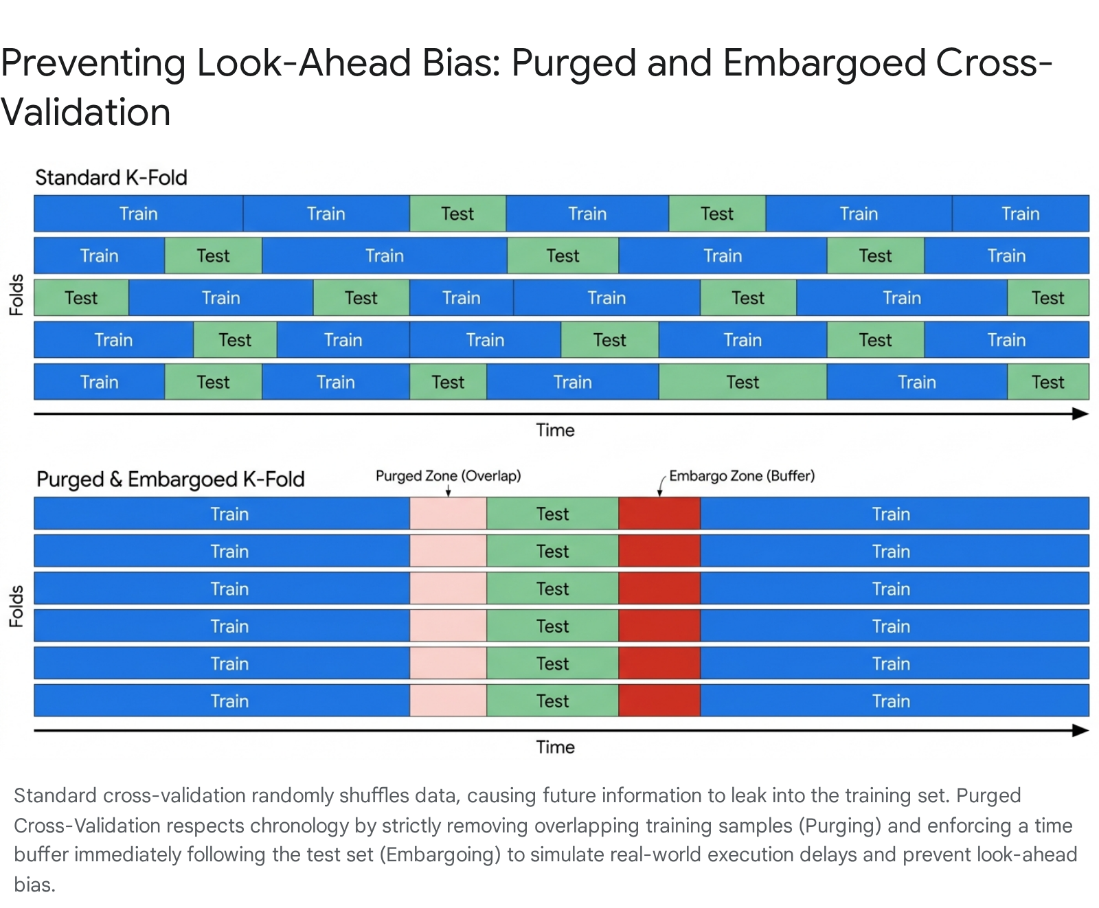
When a trading strategy evaluates a position, the outcome - the label the machine learning model is trying to predict - often spans multiple days. For example, the model may wait to see if a trade hits a 5% profit target or triggers a 2% stop loss over a ten-day horizon. Because these labels extend into the future, their horizons overlap with subsequent data points.
Purging addresses the overlap prior to the test set. If a training sample's label evaluation period overlaps in time with the beginning of the test set, that training sample must be completely purged from the dataset 54957. This removal guarantees that no observation in the training set contains information that is concurrently being evaluated in the test set, thereby preventing the model from inferring the test set's outcome 95658.
Embargoing addresses the overlap following the test set. Financial markets exhibit intense serial correlation; a massive volatility shock on a Tuesday directly dictates market behavior on Wednesday. If the training data resumes immediately on the exact day the test set ends, the model can deduce what happened during the test set simply by observing the immediate aftermath. Embargoing enforces a strict temporal buffer - often defined as a fixed number of days or a set percentage of the dataset - immediately after the test set 5495657. This buffer simulates real-world execution lags and information diffusion, entirely excluding those days from the training data 545658. If a retail algorithmic bot is backtested without rigorous purging and embargoing, its reported win rate is a mathematical illusion 54.
Are Transformers and Deep Learning Better Than Gradient Boosting in Finance?
Given the meteoric rise of generative AI and foundation models, there is an intense industry trend toward applying Transformer architectures and deep neural networks to financial time series forecasting 175960. However, empirical research from 2024 and 2025 reveals a surprising counter-narrative: for standard directional prediction on typical financial datasets, gradient boosting algorithms like XGBoost and LightGBM consistently outperform Long Short-Term Memory (LSTM) networks and vanilla Transformers 1761.
Transformers and LSTMs excel at finding complex, long-range sequential patterns in massive, highly structured data environments with rich underlying logic, such as natural language processing or protein folding 17. Financial time series data is the exact opposite. It suffers from pervasive non-stationarity, shifting macroeconomic regimes, and a notoriously low signal-to-noise ratio 176162.
Furthermore, financial prediction is effectively a tabular problem in disguise 17. When a quantitative developer calculates an RSI(14) or a 20-day ATR, they have already performed the necessary temporal sequence aggregation. The historical sequence information is mathematically compressed and baked directly into the current row of features 17. Feeding these pre-engineered features into an LSTM forces the model to pay immense computational parameter costs to search for sequential dependencies that have already been flattened into a tabular format 17. XGBoost, which excels at finding complex, non-linear relationships in tabular data, regularizes beautifully at this scale. It prevents the catastrophic overfitting that plagues deep neural networks in noisy financial environments, requires far less hyperparameter tuning, and trains at a fraction of the computational cost 917.
The Exception: The Momentum Transformer and Foundation Models
While XGBoost remains the undisputed king of tabular financial features, cutting-edge hybrid deep learning models are finding highly specialized niches where they outperform traditional techniques. Recent research in 2024 regarding the Momentum Transformer demonstrated that by combining the sequential memory of an LSTM with the attention mechanism of a Temporal Fusion Transformer, deep learning models can be forced to capture long-term macroeconomic dependencies 636465.
The architecture developed by Wood et al. utilizes a Decoder-Only Temporal Fusion Transformer that feeds an LSTM encoding layer through a Variable Selection Network, which filters out variables with low signal rates 6365. By extending the attention mechanism's lookback window to 378 days (roughly 1.5 years of trading data), the Momentum Transformer successfully navigated periods of extreme market turmoil, such as the COVID-19 pandemic, where traditional time-series momentum and mean-reversion strategies suffered severe drawdowns 636465. This hybrid design allows the model to adapt to evolving market conditions dynamically, achieving a Sharpe ratio that remained resilient even when traditional strategies inverted 6365.
Additionally, the frontier of institutional quantitative finance is moving toward using Transformers not directly for prediction, but for advanced feature engineering 5960. Rather than relying solely on manually crafted technical indicators, institutions are pre-training Transformer foundation models on massive logs of unstructured payment data, tick-by-tick order book updates, and macroeconomic text 5960. These Transformers extract "embeddings" - dense vector representations of complex market behavior 5960. These embeddings capture weak behavioral signals - the "whispers" of the market that precede major shifts - which are then fed alongside traditional tabular features into an XGBoost classifier for the final prediction 95960. This hybrid approach leverages the sequential pattern recognition of deep learning with the tabular robustness of gradient boosting.
What Are the Practical Takeaways for Hobbyist Algorithmic Traders?
For the independent developer or hobbyist aiming to survive in a market dominated by institutional supercomputers and algorithmic trading desks, success lies in rigorous data processing rather than chasing the latest complex model architecture. The empirical data dictates a strict protocol for building resilient trading systems.
First, prioritize feature engineering over algorithm selection. Spending weeks hyperparameter tuning a deep learning model yields marginal, incremental gains. Conversely, transforming raw, noisy data into high-quality, normalized features yields exponential improvements in predictive accuracy 9. A simple Logistic Regression model fed superior features will consistently outperform a poorly fed neural network.
Second, never feed raw prices into a predictive model. Apply fractional differentiation to find the optimal $d^*$ value that allows the price series to pass the Augmented Dickey-Fuller test for stationarity while maintaining the maximum possible historical memory 5222330.
Third, contextualize all technical indicators before model ingestion. Avoid the kitchen sink approach of stacking redundant momentum indicators. Ensure every selected indicator is normalized and orthogonal. Convert unbounded absolute values, such as the MACD or ATR, into percentage ratios or Z-scores so their magnitudes are contextually meaningful across shifting asset price regimes 3353742.
Fourth, scale features meticulously. If utilizing distance-based algorithms or neural networks, carefully scale features to uniform ranges using Robust Scaling or Standardization to prevent features with large numerical magnitudes from disproportionately dominating the loss function 4548. To prevent data leakage, always fit the scaler exclusively on the training data, applying that fitted transformation to the validation and test sets 3750.
Fifth, enforce rigorous cross-validation. Never use standard K-Fold cross-validation for time series analysis. Implement Purged and Embargoed Cross-Validation to guarantee that the model is evaluated strictly out-of-sample, without the artificial benefit of execution overlap or serially correlated market shocks 54956.
Finally, respect the inherent noise of the financial markets. Understand that financial data is characterized by an incredibly low signal-to-noise ratio. Begin with simpler, highly regularized tree-based models like Random Forests or XGBoost to establish a baseline before attempting to train fragile, computationally expensive deep learning architectures 1761.
Bottom line The path to profitable algorithmic trading does not run through the complexity of the neural network, but through the purity of the data pipeline. Retail traders fail at staggering rates because they assume machine learning models can magically decipher raw, non-stationary market data. By engineering memory-preserving, stationary features, applying rigorous mathematical scaling, and immunizing backtests against look-ahead bias through purged cross-validation, developers can strip away the noise of the market and isolate the faint but genuine signals of statistical edge. Models are merely the engines of prediction; disciplined feature engineering is the required fuel.