Feature Importance and Explainable AI in Trading Models
Theoretical Foundations of Explainability
The application of machine learning within quantitative finance has transitioned from linear econometric formulations to highly complex, non-linear function approximators, such as deep neural networks and gradient boosting ensembles 1. While these algorithms exhibit superior pattern recognition capabilities in high-dimensional financial data, their adoption is heavily constrained by epistemic opacity 12. The inability to trace the logic driving a model's buy or sell signal presents severe regulatory and operational risks. Explainable Artificial Intelligence (XAI) has emerged as a necessary layer in algorithmic trading, with SHapley Additive exPlanations (SHAP) achieving widespread prominence 34.
The foundational premise of SHAP rests on the Shapley value, introduced by Lloyd Shapley in 1953 to solve the problem of equitable payout distribution among players in a cooperative game 35. In machine learning, the prediction task for a single data instance represents the game, the difference between the actual prediction and the average baseline prediction represents the payout, and the input features represent the players 35. The exact Shapley value is the weighted average of a feature's marginal contributions over all permutations of feature orderings 456.
Lundberg and Lee demonstrated that Shapley values are the only attribution method that simultaneously satisfies three critical axioms 56. First, the local accuracy axiom requires that the sum of the feature attributions equals the difference between the specific prediction and the global average prediction 57. Second, the missingness axiom mandates that a feature exerting no impact across any subset receives an attribution of zero 57. Third, the consistency axiom ensures that if a model changes such that a feature's marginal contribution increases or remains static, its Shapley value cannot decrease 45.
Comparative Attribution Methodologies
To evaluate SHAP's validity in trading models, it must be contextualized against alternative frameworks, notably Permutation Feature Importance (PFI) and Local Interpretable Model-agnostic Explanations (LIME). Permutation Feature Importance, often implemented as Mean Decrease in Accuracy (MDA), evaluates a feature's macro-level importance by measuring the degradation in out-of-sample performance when the values of that feature are randomly shuffled 89. This approach breaks the relationship between the feature and the target variable but fails to provide instance-level explanations for specific trades 10.
Conversely, LIME isolates an individual prediction and generates a local surrogate model - typically a linear regression - trained on a synthetic dataset created by perturbing the input features around the instance of interest 101112. While providing localized interpretability, LIME relies on linear approximations and struggles to faithfully capture highly complex, non-linear feature interactions if the decision boundary is jagged within the local neighborhood 1314.
| Attribution Methodology | Scope of Evaluation | Treatment of Feature Interactions | Stability and Consistency Metrics |
|---|---|---|---|
| SHAP (TreeSHAP/KernelSHAP) | Global and Local | Captures non-linear interactions across all possible coalitions via cooperative game theory. | High. Mathematically guarantees consistency and satisfies local accuracy axioms 57. |
| Permutation Importance (PFI / MDA) | Global only | Ignores synergistic interactions; penalizes features individually based on performance drop. | Low. Highly sensitive to the random seed used during the validation permutation 1516. |
| LIME | Local only | Uses a linear surrogate; struggles with deep non-linear feature interactions in complex spaces. | Moderate. Stability varies depending on the perturbation sampling method and variance 11. |
Table 1: Comparative Analysis of Feature Importance Methodologies in Quantitative Finance.
Mathematical Mechanics of Feature Attribution
Approximating exact Shapley values in high-dimensional financial environments is computationally intractable, leading to the development of specialized estimation algorithms. TreeSHAP provides a rapid, exact calculation specifically optimized for tree-based models like Random Forests and XGBoost, transforming the exponential complexity of standard Shapley calculations into polynomial time by leveraging the internal structure of the decision trees 314. For neural networks and model-agnostic applications, KernelSHAP and DeepSHAP rely on weighted linear regression and layer-wise propagation, respectively, to estimate feature contributions relative to a background dataset 514.
Multilinear Sampling and Interaction Indices
To further improve the computational efficiency of Shapley value estimation, researchers have introduced multilinear sampling algorithms. By applying multilinear extension techniques from game theory, specific sampling methods significantly reduce the variance of the sampling statistics for models like Multilayer Perceptrons (MLPs), outperforming traditional Owen sampling mechanisms 18.
Furthermore, standard Shapley values quantify individual feature contributions but do not explicitly isolate interaction effects. Advancements such as the Faithful Shapley Interaction Index (Faith-Shap) define the family of interaction indices that satisfy interaction-extended Shapley axioms without requiring less-intuitive assumptions 17. By formulating interactions through weighted polynomial regression, Faith-Shap captures complex dependencies - such as the synergistic effect between a momentum indicator and a volatility regime - providing a formal axiomatic guarantee for interaction attribution 17.
Multicollinearity and the Substitution Effect
Financial market data is inherently characterized by dense multicollinearity. Quantitative models predicting asset returns frequently ingest overlapping features, such as multiple moving average crossovers, various formulations of the Relative Strength Index (RSI), and correlated macroeconomic indicators 181920. The presence of highly correlated variables introduces structural challenges for feature attribution, fundamentally altering how models assign predictive weight.
Attribution Dilution and Feature Splitting
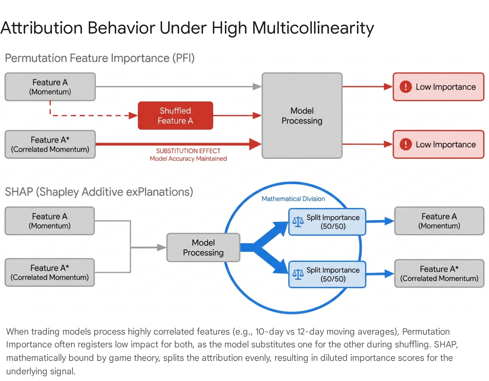
When multiple features encode similar informational signals, models exhibit a substitution effect 21. If one feature is unavailable, the algorithm relies on a substitute feature without a significant loss in accuracy. This collinearity disrupts the baseline intuition of permutation algorithms. In PFI, shuffling one highly correlated feature while leaving its substitute intact often results in negligible performance degradation, causing the algorithm to assign artificially low importance to both variables 910.
SHAP addresses multicollinearity through cooperative credit splitting. Because Shapley values evaluate all possible feature coalitions, identical information provided by two correlated variables is mathematically split between them 18. While this satisfies game-theoretic fairness, it causes attribution dilution in trading models. A dominant underlying signal, such as cross-sectional momentum, may appear artificially weak in a global SHAP summary plot because its importance has been fractured across a dozen separate momentum indicators 922.
Pre-processing and Mitigation Techniques
To ensure attribution scores reflect actual market drivers, researchers must actively manage multicollinearity prior to applying XAI. Standard protocols utilize the Variance Inflation Factor (VIF), recursively filtering out features with VIF scores exceeding conservative thresholds (e.g., VIF > 5 or 10) to force models to rely on orthogonal data 202324.
When structural feature sets cannot be pruned, advanced frameworks such as Vector SHAP and Group Shapley are implemented 2528. Group Shapley extends the classical framework by evaluating the importance of clustered blocks of variables - such as grouping all short-term liquidity metrics into a single game-theoretic entity 25. This avoids attribution dilution and yields a statistically robust evaluation of broader macroeconomic or fundamental factors, validated by testing procedures that handle sparse distributions using three-cumulant chi-square approximations 25.
Out-of-Sample Robustness and Stability Metrics
The validity of algorithmic trading models relies on out-of-sample robustness - the capacity to generalize to unseen data under varying market regimes 1. Interpretability algorithms face parallel requirements. An explanation generated by an XAI method is operationally invalid if slight data perturbations or differing random seeds yield entirely contradictory feature importance hierarchies 1526.
Quantifying the Instability Index
Stability is formally evaluated using the instability index, which quantifies the variance of a feature's rank across multiple executions 1516. Permutation Importance displays acute instability due to its stochastic row-shuffling mechanics 1521. Although expanding the iteration count reduces this variance, the instability index for MDA in empirical financial datasets never converges to zero 15.
LIME and SHAP demonstrate substantially higher stability 1516. While KernelSHAP exhibits variability dependent on the size of the background dataset 1113, exact algorithms like TreeSHAP eliminate seed variance. Rank verification algorithms, such as SPRT-SHAP and RankSHAP, perform retrospective analysis on estimated Shapley values to formally verify global importance rankings with statistical confidence bounds 6.
To quantify uncertainty in explanations, Bayesian-AIME treats feature attribution probabilistically, yielding 95% credible intervals for each feature's importance 2627. Similarly, Complexity and feature interaction-adjusted SHAP (CESHAP) mathematically isolates and mitigates distortions caused by random noise in tree-based models, establishing highly robust attributions even across non-linear market environments 8. Additional regularization techniques, such as SHAP entropy penalties, force machine learning models to rely on sparse, stable distributions of features during the training phase itself 31.
Feature Selection and Generalization Efficacy
Despite approximation variances, utilizing SHAP for feature selection significantly improves out-of-sample predictive performance 153233. In a study analyzing an equity strategy across 464 historical trades, applying feature selection methods elevated the strategy's baseline Sharpe ratio from 0.36 to 0.83, simultaneously doubling cumulative returns 15.
Empirical research in specific asset markets confirms these findings. An evaluation of the top five high-volume banks in the Turkish BIST100 index during a high-inflation regime utilized SHAP to filter inputs for an ARIMA-LSTM hybrid model 1819. The SHAP-filtered model systematically discarded noise, revealing a dominant reliance on lagged momentum indicators (RSI) and trading volume, ultimately generating robust walk-forward predictions 1819. In similar telecommunications churn datasets, SHAP feature reduction achieved a Spearman rank correlation of $\rho = 0.94$ with baseline permutation methods while reducing dimensionality by 20% and preserving predictive F1-scores 32.
Temporal Dynamics and Look-Ahead Bias
Applying explainable AI to financial time-series forecasting introduces severe methodological risks, most notably look-ahead bias 2829. Look-ahead bias occurs when a model implicitly or explicitly accesses information that was not available at the historical moment the trading decision was generated 2830.
Background Dataset Mechanics and Leakage
To evaluate marginal feature contributions, SHAP must simulate the absence of a feature by marginalizing over a background dataset 51137. The statistical distribution of this background sample establishes the baseline expectation against which the specific instance is compared 51131.
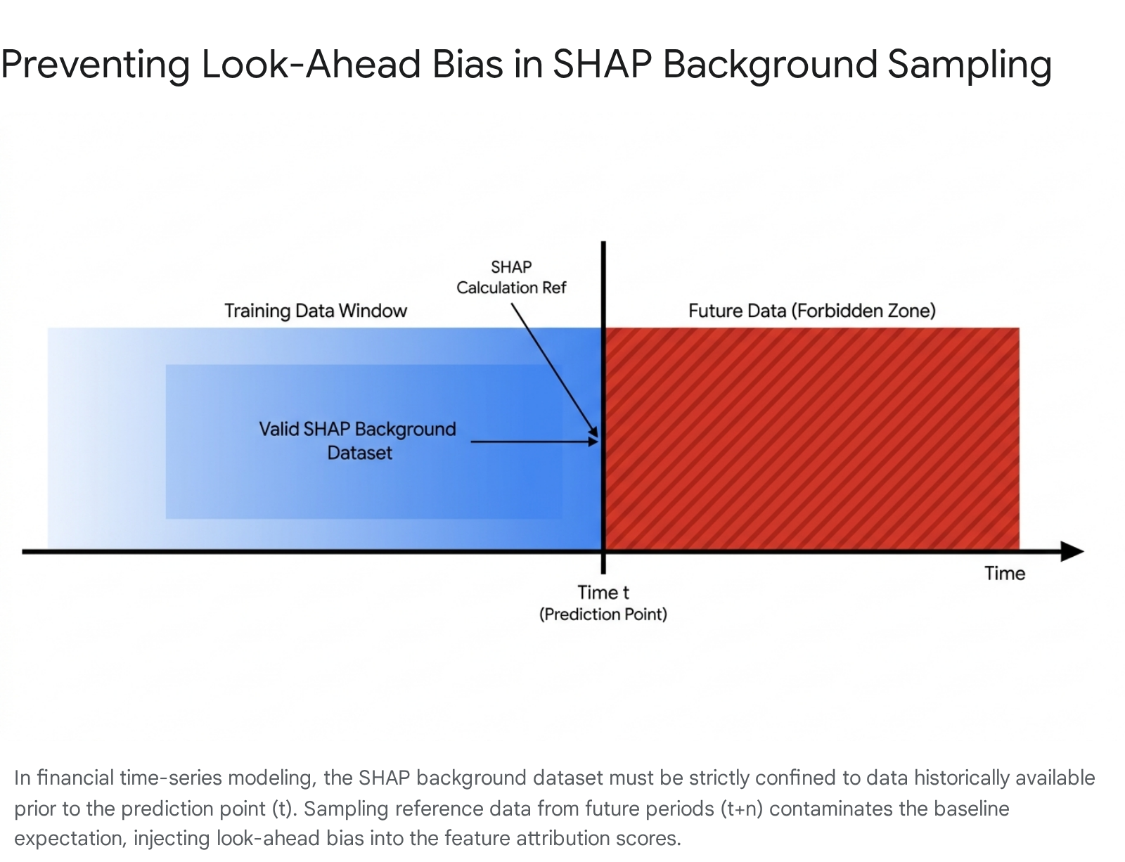
In standard cross-sectional machine learning, randomly sampling the training data to form this background is standard practice 1332. In finance, random sampling destroys temporal integrity 2931. If an analyst queries SHAP to explain an algorithmic trade made in 2021, and the background dataset randomly includes market data from 2023, the algorithm is explicitly leaking future volatility distributions into the baseline calculation 2931. The resulting SHAP attribution will measure the 2021 trade's logic relative to an environment that did not yet exist.
Maintaining Structural Validity
To immunize SHAP against temporal data leakage, quantitative pipelines must enforce strict chronological partitioning 2933. Researchers analyzing US macroeconomic metrics enforce initial gaps between training and testing sets to prevent multi-month forecasts from overlapping with validation vectors 31.
Background datasets must utilize a rolling, expanding window framework 2933. The reference data used to evaluate a given prediction must consist entirely of observations occurring chronologically prior to the execution timestamp 2933. Because market regimes continuously shift, the background distribution must also be updated frequently to ensure the baseline accurately reflects the prevailing liquidity and volatility environment, rather than stale, multi-year averages 1031.
The Illusion of Causality and Narrative Bias
While SHAP solves the technical problem of attributing predictive weight, it exacerbates a fundamental cognitive vulnerability in analysts: narrative bias 413435. In quantitative research, SHAP values are frequently misinterpreted as causal proofs, leading to the construction of post-hoc financial stories that are not mathematically supported by the data.
Associational Mappings versus Causal Structures
The primary epistemological failure in deploying SHAP lies in confounding associational feature importance with causal intervention 3235. SHAP provides predictive attribution; it quantifies how observing a specific feature value shifts the algorithm's output 32. It does not provide causal identification 323536.
In formal causal inference, such as Pearl's Directed Acyclic Graphs (DAGs) and the do-calculus, the statement "X causes Y" signifies that a deliberate intervention on X will predictably alter Y 37. In contrast, observing a high SHAP value for feature X merely indicates that X serves as an effective statistical proxy for estimating Y 353637. For example, SHAP dependence plots may demonstrate a strong directional mapping where increased return volatility heavily influences a deep learning model's forecast. Analysts frequently mistake this directional sensitivity for causality, concluding that the volatility directly drove the asset price 35. In reality, both the volatility and the price movement may be downstream symptoms of an unobserved confounding variable, such as an institutional liquidity shock 3637.
Academic literature categorizes these errors as Type-A and Type-B spurious claims - strategies built on historical associations without formalized causal mechanisms or falsification criteria 37. Validating an algorithmic signal with SHAP does not convert a correlational model into a causal one; it merely visualizes the historical correlations the algorithm has memorized 3537.
Cognitive Framing and Financial Storytelling
Narrative bias is the human predisposition to impose structured, cause-and-effect reasoning onto ambiguous, purely correlational data streams 413438. The field of narrative economics, advanced by Robert Shiller, demonstrates how collective stories - such as the viral retail narratives surrounding meme stocks (e.g., GameStop, AMC) or post-COVID inflation expectations - exert independent influence on market fundamentals by coordinating mass behavior 3439.
When analysts review SHAP output, they often succumb to this exact bias. Presented with a vector of weights indicating that short-term momentum and bid-ask spread were highly impactful for a specific trade, the analyst constructs a logical, post-hoc story: "The model detected a short-squeeze setup and traded the momentum breakout" 2834. The machine learning model engaged in no such reasoning; it executed a complex matrix optimization process devoid of economic comprehension 4840. SHAP inadvertently supplies the quantitative vocabulary required for analysts to craft convincing, yet spurious, justifications for algorithmic behavior 303841.
Parallels in Epidemiological Observational Data
The risks of narrative bias observed in financial AI parallel established systemic issues in epidemiological research. In medical literature, researchers evaluating observational health data frequently misattribute correlation to causation, overlooking critical confounding variables 42. Analyzing data without a strict causal framework results in "spin" - the use of emotional rhetoric, biased numerical framing, and oversimplification to exaggerate non-significant findings or imply definitive causality where none exists 42434454.
When visual data representations and contextual storytelling are combined, readers demonstrably struggle to detect underlying causal fallacies 3442. Just as narrative framing in medical abstracts misleads healthcare policy decisions 4354, narrative bias in quantitative finance leads portfolio managers to over-allocate risk to models that are statistically brittle but conceptually persuasive 3445.
Structural Validity Frameworks in Algorithmic Trading
To operationalize XAI without succumbing to narrative fallacy, financial institutions are deploying strict structural validity frameworks 2830. Research identifying critical vulnerabilities in financial AI integration highlights five pervasive biases that contaminate strategy backtests:
| Classification | Definition of Bias in Financial Modeling |
|---|---|
| Look-ahead Bias | Utilizing data that did not exist at the historical time of the decision, either through direct input or temporal leakage in background datasets 282930. |
| Survivorship Bias | Restricting the evaluation universe to entities that survived the entire testing period, artificially inflating historical returns by ignoring delisted or bankrupt assets 2830. |
| Narrative Bias | The generation of a coherent, post-hoc rationale for an algorithm's output that is not fundamentally supported by the evidence available at execution time 2830. |
| Objective Bias | Training systems to prioritize confident, definitive completions rather than outputting calibrated uncertainty or safe refusal when signal noise is overwhelming 2830. |
| Cost Bias | Reporting gross theoretical performance while ignoring market friction, slippage, bid-ask spread, and realistic trade execution costs 2830. |
Table 2: The Five Critical Biases in Financial Machine Learning Applications.
To neutralize these biases, explainability must be integrated iteratively into the research lifecycle rather than appended as a post-trade justification tool 3256. For example, the Context-Enriched Agentic RAG (CARAG) framework explicitly mitigates monolithic narrative bias by employing cooperative sub-agents that cross-reference historical performance, corporate guidance, and peer benchmarks to prevent an AI model from merely parroting optimistic management sentiment during earnings calls 41.
In portfolio management, SHAP is optimally deployed to monitor concept drift and maintain algorithmic governance 5657. If longitudinal tracking of global SHAP values reveals that a model's reliance has suddenly shifted from long-term volatility metrics to transient intraday order flow, risk managers can halt trading and recalibrate the system before out-of-sample degradation occurs 1028. By decoupling XAI from storytelling and leveraging it strictly as an audit mechanism for feature stability, practitioners extract genuine, actionable signal from complex models 2257.