Meta-labeling and triple-barrier methods in machine learning trading
Foundational Challenges in Financial Signal Generation
The application of machine learning to financial markets requires domain-specific adaptations to overcome the unique structural challenges of financial time series data. Traditional machine learning techniques, originally developed for static cross-sectional data or clean, stationary temporal sequences, often fail when applied directly to market data 12. Financial markets are characterized by high noise-to-signal ratios, non-stationarity, shifting volatility regimes, and complex microstructural frictions 34. Marcos López de Prado has extensively documented that standard data science methodologies, when applied to quantitative finance, routinely lead to backtest overfitting and the deployment of false strategies 23.
Historically, quantitative researchers have relied on fixed-time horizon methods to generate targets for supervised learning algorithms. In a fixed-horizon framework, an observation at time $t$ is labeled based on the asset's return at a fixed future point, $t+h$ 784. While computationally simple and common in academic literature, this approach inherently ignores the path the price takes between the time of the signal and the evaluation horizon. In live trading, a position may experience extreme volatility, triggering a margin call or exceeding risk tolerance long before the evaluation horizon is reached 81011. Consequently, models trained on fixed-horizon labels often exhibit poor out-of-sample generalization, failing to account for practical trading constraints such as stop-loss mechanisms and holding costs 81011.
To address the disconnect between academic machine learning and practical trading realities, researchers have introduced advanced data structuring, labeling, and modeling paradigms. Chief among these are the triple-barrier method for realistic outcome labeling and meta-labeling architectures for dynamic position sizing and false-positive suppression 27513. These techniques shift the objective of financial machine learning from merely predicting absolute price direction to probabilistically evaluating the reliability and execution viability of trading signals under real-world constraints.
Information-Driven Data Structures
Before complex labeling mechanisms can be applied effectively, the underlying market data must be sampled in a manner that preserves statistical integrity. Traditional financial models utilize time-based bars, sampling data at fixed intervals such as end-of-day, 5-minute, or 1-hour periods 41415. Time bars suffer from severe statistical flaws; they oversample periods of low market activity and undersample periods of high activity, leading to statistical properties that violate the independent and identically distributed (IID) assumptions of many machine learning algorithms 10146.
Information-driven sampling algorithms, such as volume bars, dollar bars, and tick bars, generate observations only when a predefined threshold of market activity is reached. Dollar bars form a new observation each time a specific fiat value of the asset is transacted 1014. This volumetric approach normalizes the data against long-term price appreciation, ensuring that the algorithm focuses its computational resources on periods where significant market microstructure events are actually occurring, rather than processing chronological noise 1114.
A further necessary refinement for event-driven trading is the Cumulative Sum (CUSUM) filter. The CUSUM filter is a quality-control sampling technique designed to detect structural breaks and significant shifts in the underlying data-generating process 4106. The filter triggers an event - and seeds a potential machine learning observation - only when the cumulative deviation of returns exceeds a dynamic, volatility-adjusted threshold 141517. By filtering out background noise and focusing strictly on informative market events, practitioners construct more robust datasets that are highly suitable for advanced labeling techniques.
Triple-Barrier Labeling Methodology
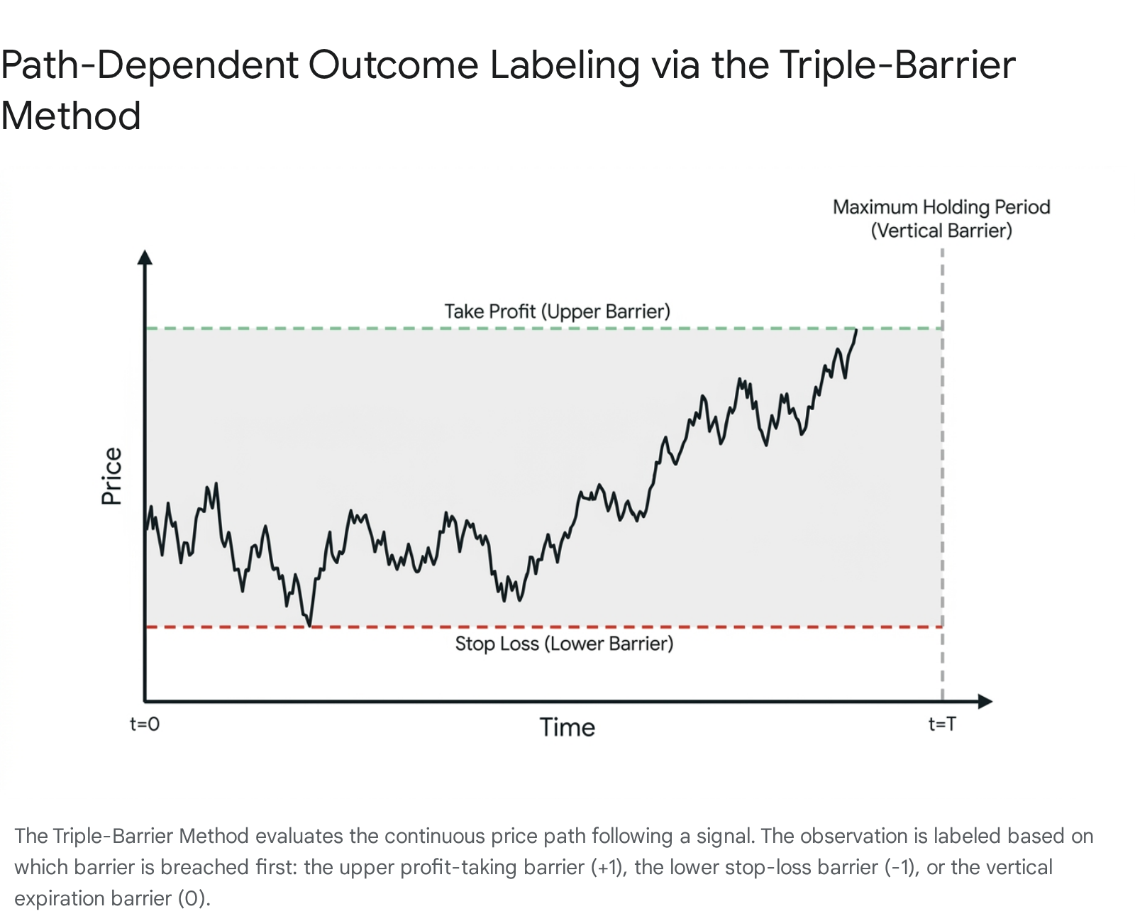
The triple-barrier method was developed to embed risk management constraints directly into the supervised learning target variable 784. Rather than asking a model to predict the arbitrary price level of an asset at a specific future time, the triple-barrier method simulates the exact mechanics of a live trade execution, factoring in the objective reality that traders employ limits to protect capital.
Mechanics of Dynamic Barriers
For any given observation triggered by a market event at time $t$, three distinct boundaries are established to define the outcome of the theoretical position: an upper barrier for profit-taking, a lower barrier for a stop-loss, and a vertical barrier representing the maximum time horizon 278. The upper barrier is set at a distance above the entry price, representing the desired profit target. The lower barrier is set at a distance below the entry price, representing the maximum acceptable loss before the trade is invalidated. Finally, the vertical barrier is set at a fixed duration after the entry time, representing the maximum holding period, which enforces capital efficiency by freeing up locked capital if a trade stagnates 278.
The target label is determined purely by identifying which of the three barriers the continuous price path intersects first. If the upper barrier is hit before the others, the observation is labeled $+1$, indicating a successful long trade. If the lower barrier is hit first, it is labeled $-1$, representing a successful short trade or a failed long trade. If the vertical barrier is breached before either horizontal barrier is touched, the observation is traditionally labeled $0$, indicating that the signal expired without sufficient directional momentum 81417.
Some implementations map these to different discrete classes (e.g., $0, 1, 2$) depending on the specific multi-class architecture of the supervised learning model being used, but the core logic remains identical 18.
Volatility Scaling and Heteroskedasticity
A critical innovation of the triple-barrier method is the dynamic scaling of the horizontal barriers based on localized market volatility 81819. Financial markets exhibit pronounced heteroskedasticity; a 1% price movement is highly significant in a low-volatility consolidation regime but constitutes standard intraday noise during a high-volatility regime or a market crash. Static thresholds fail to account for these structural shifts, resulting in excessive stop-outs during volatile periods and unreached profit targets during quiet periods.
To correct this, the barriers are computed as a function of point-in-time volatility, often estimated via an exponentially weighted moving average of standard deviations or average true range (ATR) computed over a rolling window 141819. The thresholds are mathematically defined as $S_t \times (1 \pm (\sigma_t \times \Delta))$, where $\sigma_t$ is the localized volatility and $\Delta$ represents a configurable multiplier for the take-profit or stop-loss limits 8. This scaling mechanism ensures that the risk-reward ratio adapts fluidly to shifting market conditions, preventing the machine learning model from generating artificially high success rates during hyper-volatile periods or suffering severe drawdowns when underlying market regimes change 11.
Embedded Execution Realities
By incorporating stop-losses and take-profits directly into the label generation process, the triple-barrier method forces the machine learning model to internalize the concept of path dependency 86. A traditional fixed-horizon model might label a trade as profitable if the closing price at the end of the week is higher than at the beginning, completely ignoring the fact that the asset's price may have dropped by 20% in the interim. In live market conditions, such an interim drop would have triggered a margin call or a manual risk-management stop-loss, realizing a loss rather than a gain 117. Triple-barrier labels accurately reflect the objective reality of trading survival, effectively teaching the algorithm how to optimize risk-adjusted returns rather than simple, but theoretically flawed, directional predictive accuracy 11.
Trend-Scanning Methodology
While the triple-barrier method excels in modeling discrete execution paths and strict risk-reward thresholds, other techniques have been developed to capture broader market dynamics where the researcher may not want to explicitly set a fixed profit or stop-loss level. Trend-scanning is a complementary labeling methodology introduced by López de Prado to identify the presence, direction, and magnitude of trends adaptively 268.
In the trend-scanning framework, multiple linear regressions are fitted over varying forward-looking windows, from time $t$ to $t+L$, where $L$ represents a maximum look-forward parameter. For each observation, the algorithm fits regressions across all possible window lengths and selects the specific time window that yields the maximum t-statistic for the slope coefficient of the regression line 6. This ensures that the label captures the most statistically significant trend, regardless of whether it concludes in three hours or three days.
This method serves dual purposes in financial machine learning pipelines. For classification tasks, the sign of the maximum t-value indicates the direction of the trend, assigning $+1$ for an upward trend and $-1$ for a downward trend. By introducing a minimum t-value threshold for statistical significance, observations that lack a definitive trend can be cleanly labeled $0$ 6. For regression tasks, the magnitude of the t-value quantifies the strength and statistical confidence of the trend. This continuous value can be utilized directly as a regression target or as sample weights in downstream classification tasks, ensuring the learning algorithm prioritizes optimization on the most pronounced and reliable market moves rather than noise 6.
While trend-scanning is highly adaptive, empirical studies indicate that it serves a different purpose than barrier methods. Trend-scanning is effective for broad regime identification and market-timing strategies that seek to sit in a position until a structural trend changes 6. However, it can struggle to handle complex, non-linear inter-asset relationships and microstructural noise in highly volatile markets when compared directly to multi-scale barrier methods that explicitly define execution limits 49.
| Feature / Methodology | Fixed-Horizon Labeling | Triple-Barrier Method | Trend-Scanning |
|---|---|---|---|
| Labeling Mechanism | Asset return measured precisely at a fixed point $t+h$. | First barrier touched (Take-profit, Stop-loss, or Time limit). | Maximum t-value of regression slopes over dynamic forward windows. |
| Path Dependency | None. Ignores inter-period price extremes. | High. Captures the exact sequence of price movements. | Moderate. Acknowledges broader trend trajectory over varying lengths. |
| Volatility Adaptation | Typically static, requiring manual adjustment across regimes. | Highly dynamic. Barriers scale directly with rolling point-in-time volatility. | Indirect. Adapts by shifting the optimal look-forward window length. |
| Primary Use Case | Baseline academic benchmarking and low-frequency forecasting. | Realistic algorithmic execution, position sizing, and risk management. | Macro trend identification, market timing, and sample weighting. |
| Microstructural Risk | Ignores slippage, stop-outs, and margin constraints entirely. | Mimics live trading environment and capital preservation logic. | Identifies structural momentum but lacks specific exit constraints. |
Meta-Labeling Architecture
Despite the adoption of advanced data sampling and robust labeling techniques, primary predictive models in finance - whether driven by fundamental analysis, technical indicators, or complex deep learning - often suffer from low precision and high false-positive rates 52324. A primary model designed to capture every possible breakout or mean-reversion event will inevitably trigger trades in suboptimal market conditions. Meta-labeling, frequently referred to as corrective AI, resolves this by decomposing the trading decision into a two-layer hierarchical architecture 5. The fundamental premise of meta-labeling is the strict separation of the directional prediction (the side of the trade) from the confidence estimation (the size of the trade) 51011.
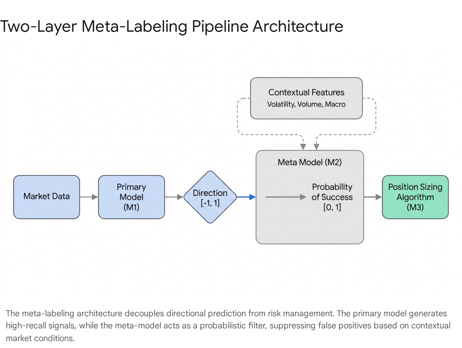
Primary Signal Generation
The primary model is responsible for generating raw trading signals. This layer does not necessarily rely on complex machine learning; it can be driven by traditional econometric models, fundamental factor analysis, moving average crossovers, statistical arbitrage spreads, or neural networks 232412. The primary model evaluates the market state and issues a directional forecast, typically proposing a long, short, or neutral position 5.
The specific design objective for the primary model is to maximize recall. In binary classification terms, recall represents the model's ability to identify as many profitable opportunities as possible, even if doing so results in a high number of false positives 613. In this first stage, missing a valid trading opportunity is viewed as a greater error than flagging a false one, because the secondary layer is specifically engineered to perform the necessary filtration.
Meta-Model and Probabilistic Filtering
The secondary model, or meta-model, acts as a sophisticated gatekeeper. It does not predict the direction of the asset; instead, it predicts whether the primary model's specific signal will be successful in the current environment. The target variable for the meta-model is strictly binary, marked as $1$ if the primary signal achieves its profit target or $0$ if it hits a stop-loss or expires 5232412. The ultimate goal of the meta-model is to maximize the F1-score of the combined system by dramatically increasing precision, acting as a filter that sacrifices some recall to eliminate low-quality trades 11613.
To make this determination, the meta-model is trained on an expanded feature set. It ingests the directional output of the primary model, but crucially, it also ingests a broad array of contextual variables that define the current market regime. These features often include point-in-time volatility metrics, bid-ask spread dynamics, market depth, order flow imbalances, macroeconomic indicators, and recent primary model performance statistics 232412.
Through supervised training on these rich features, the meta-model learns complex, non-linear relationships indicating when the primary strategy tends to fail. For example, a momentum-based primary model may perform exceptionally well in trending environments but suffer severe drawdowns during mean-reverting, low-liquidity regimes. The meta-model detects these structural conditions and outputs a low probability score, effectively suppressing the trade before capital is deployed 42324.
Probability Calibration and Position Sizing
The direct output of the meta-model is a probability estimate representing the system's confidence in the trade's success 5. However, raw probabilities generated by complex machine learning classifiers - such as Random Forests, Support Vector Machines, or Gradient Boosting models - are often miscalibrated. They do not accurately reflect the true posterior probability of the event occurring, frequently clustering probabilities near the extremes or the mean 1014.
Before executing a trade and allocating capital, probability calibration techniques are applied to ensure the model's confidence scores align with empirical win rates. Research indicates that the performance of fixed position sizing methods is significantly improved by proper calibration 101415. Techniques such as Platt scaling or isotonic regression map the raw outputs to calibrated probabilities, resulting in more stable metrics and significantly lower maximum drawdowns 14.
Once calibrated, these probabilities are fed into a position sizing algorithm. Established methods include linear scaling, optimal Kelly criterion applications, and Sigmoid Optimal Position Sizing (SOPS). If the meta-model expresses high confidence, the system allocates a larger capital position. If the confidence approaches the 0.5 threshold - indicating a coin-toss probability of success - the allocation scales down toward zero 51014. This continuous scaling acts as a dynamic risk control mechanism, preserving capital during unfavorable regimes and aggressively deploying it when conditions strongly align with the strategy's core edge.
Architectural Variations and Ensembles
As the meta-labeling framework has matured in professional quantitative finance, researchers have developed heterogeneous architectures to optimize the filtering mechanism for specific trading strategies and asset classes 510.
Recognizing that the microstructural dynamics driving upward price action often differ fundamentally from those driving downward action - due to factors like short-selling restrictions, differing margin requirements, and asymmetric risk aversion - practitioners often employ Discrete Long and Short architectures. This approach splits meta-labeling into two specialized secondary models: one explicitly trained to evaluate long signals, and another to evaluate short signals, thereby improving overall classification accuracy and reducing noise 512.
Another variation is Conditional Meta-Labeling (CMLA). This architecture explicitly partitions historical data based on predefined market regimes, such as high versus low volatility or economic expansion versus recession. Specialized meta-models are then trained independently for each specific condition. During live trading, the system routes the primary signal to the condition-specific meta-model best suited to evaluate it 5.
Finally, individual machine learning classifiers possess distinct strengths and biases. Ensemble Meta-Labeling aggregates predictions from diverse base models - such as Logistic Regression, Gradient Boosting Machines, and Support Vector Machines - using a meta-learner to fuse their probability outputs. Systematic studies demonstrate that ensemble meta-labeling significantly improves regime detection, reduces false-positive rates, and enhances generalization performance across highly imbalanced financial datasets 103116.
Empirical Performance Across Asset Classes
The theoretical advantages of triple-barrier labeling and meta-labeling translate into significant, quantifiable improvements in out-of-sample trading performance across diverse asset classes. Empirical studies demonstrate that the primary benefit of meta-labeling is not the maximization of absolute returns, but the dramatic improvement in risk-adjusted metrics - specifically the Sharpe ratio, Calmar ratio, and maximum drawdown 23241718.
Equity Markets and Traditional Assets
In controlled experiments applied to S&P 500 E-mini futures and equity indices, the integration of meta-labeling consistently upgrades baseline strategies by acting as a highly effective filter. When evaluating mean-reverting strategies, such as those based on Bollinger Bands, researchers found that applying meta-labeling improved the classification accuracy of a baseline model from 20% to 77% in validation sets, and from 17% to 63% in completely out-of-sample test sets 1719. For trend-following strategies tested under similar parameters, accuracy jumped from 37% to 56% in validation and from 48% to 55% out-of-sample, translating to improved strategy performance metrics 1719.
By surgically removing low-confidence trades, meta-labeling severely curtails the left tail of the return distribution. Researchers report that sacrificing raw recall to maximize precision results in fewer severe drawdowns, allowing for higher geometric compounding over time 232420. A highly optimized quantitative equity strategy leveraging hierarchical risk parity, multi-horizon XGBoost ensembles for meta-labeling, and regime gating achieved a verified out-of-sample Sharpe Ratio of 2.06. This strategy limited its maximum drawdown to just -11.6% while simulating full margin interest and linear slippage, demonstrating the robustness of the layered architecture 20.
| Strategy Type | Baseline Accuracy (OOS) | Meta-Labeled Accuracy (OOS) | Relative Improvement |
|---|---|---|---|
| Mean-Reverting (S&P 500) | 17.0% | 63.0% | +270% |
| Trend-Following (S&P 500) | 48.0% | 55.0% | +14% |
| Hybrid Ensemble (Multi-factor) | Low Precision | High F1-Score | Significant Drawdown Reduction |
High-Volatility Environments and Cryptocurrency
Cryptocurrency markets present a severe test for financial machine learning models due to their extreme volatility, persistent inefficiency, and frequent structural breaks. Traditional fixed-horizon methods routinely fail in these environments, as the massive intraday price swings trigger unseen drawdowns that fixed-point evaluation ignores 4.
In a comprehensive 2025 study evaluating deep learning architectures across Bitcoin and Ethereum, researchers combined CUSUM-filtered data with triple-barrier labeling to navigate the market's noise. The performance divergence between baseline methods and the advanced architecture highlighted the necessity of dynamic boundaries 15. The deep learning hybrid models using triple-barrier labeling achieved robust risk-adjusted returns compared to negative baseline returns over the testing period.
| Methodology / Asset | Ethereum (ETHUSDT) Annualized Sharpe | Bitcoin (BTCUSDT) Annualized Sharpe | Max Drawdown (ETH) |
|---|---|---|---|
| Traditional Buy & Hold | Negative Return (-44%) | Negative Return (-34%) | > 50% |
| Fixed Horizon Baseline | -0.29 | -0.29 | High |
| Trend Scanning Baseline | 0.00 | 0.00 | High |
| TBM + CUSUM (2% threshold) | 1.42 | 0.51 | 25.1% |
| TBM + Range Bars (3% threshold) | 1.44 | N/A | 10.7% |
The application of model-agnostic meta-learning and multi-scale causal inference frameworks has further pushed these boundaries. An Adaptive Event-Driven Labeling framework tested across 16 assets over a 25-year span achieved an average Sharpe ratio of 0.48, compared to near-zero or negative performance for standard baselines (Fixed Horizon: -0.29, Triple Barrier baseline: -0.03, Trend Scanning: 0.00) 49. Ablation studies in this research revealed that judicious component selection is vital; relying purely on the multi-scale barrier dynamics without overly rigid causal filtering actually improved the Sharpe ratio to 0.65 across all assets. This indicates that while algorithmic complexity can aid prediction, the core mechanics of risk-aware barrier labeling drive the bulk of the sustained edge 49.
Integration with Advanced Machine Learning Architectures
The quantitative finance industry is currently witnessing a rapid convergence of meta-labeling philosophies with frontier deep reinforcement learning (DRL) and Transformer network architectures 21. Reinforcement learning naturally models the sequential, path-dependent nature of trading, seeking to maximize a reward function over an extended episode rather than minimizing static classification errors 3839.
In recent research exploring Foreign Exchange trading, researchers designed a two-part reinforcement learning system directly inspired by the meta-labeling framework. This Entropy-Regulated Lagrangian (ERL) approach decoupled tasks into two specialized agents: a Directional Agent utilizing Proximal Policy Optimization (PPO) with Long Short-Term Memory (LSTM) layers, and a Meta-labeling Agent responsible for determining trade entry, position sizing, and dynamic take-profit/stop-loss levels 38.
This decoupled RL architecture achieved a 38.11% cumulative return on out-of-sample data, maintaining a Sortino ratio of 0.0905, which was higher than its Sharpe ratio of 0.0660. The elevated Sortino ratio indicates that the system's volatility was predominantly driven by upside gains rather than downside losses. Furthermore, the Calmar ratio reached 1.36 against a maximum drawdown of -28.03%, demonstrating strong risk-adjusted performance in a notoriously difficult asset class 38.
Simultaneously, Transformer networks - recognized for their self-attention mechanisms and ability to process long-range temporal dependencies without the vanishing gradient problems of traditional sequential models - are being fine-tuned on meta-labeled financial datasets. Models such as the Momentum Transformer learn to prioritize the most relevant historical sequences, integrating structural cues like fair value gaps, order block inefficiencies, and volatility regimes to generate highly robust, multi-horizon forecasts that outperform traditional LSTM approaches 22412324.
Market Frictions and Execution Realities
A model demonstrating high theoretical predictive accuracy is irrelevant if its statistical edge is consumed by market microstructure frictions. In high-frequency and medium-frequency trading environments, transaction costs, bid-ask spreads, and execution slippage - the difference between the expected price of a trade and the actual execution price - can rapidly turn a profitable paper strategy into a net loser 24252627. Research on portfolio optimization highlights that transaction costs can reduce annual returns by 0.5% to 2% depending on trading frequency, making the management of portfolio turnover a critical component of algorithmic success 27.
Standard machine learning models optimized purely for statistical loss metrics tend to overtrade. Because they lack an understanding of execution drag, they treat all predicted signals equally, initiating positions regardless of the expected magnitude of the price move or the current liquidity profile of the order book 2527. The Drawdown Dichotomy Ratio (DDR), a metric quantifying the structural gap between floating risk and realized risk, highlights how theoretical maximum drawdowns can vastly underestimate true capital exposure when slippage and consecutive micro-losses accumulate 7.
Meta-labeling structurally mitigates the impact of these transaction costs through conditional execution. By assigning confidence probabilities to primary signals, the meta-model establishes a rigid mathematical threshold for action. Low-confidence signals - which represent a high proportion of a primary model's output in noisy, mean-reverting markets - are systematically rejected. This filtration process drastically reduces unnecessary portfolio turnover. Consequently, the strategy only pays the bid-ask spread and incurs execution slippage on high-probability setups where the expected profit margin significantly outweighs the microstructural drag 232438.
Furthermore, incorporating the triple-barrier method ensures that the training data explicitly reflects these economic constraints. The horizontal profit-taking and stop-loss barriers can be defined to account for the minimum required profit margins necessary to clear execution costs. If a price path does not breach this cost-adjusted upper barrier, the trade is marked as a failure during the model's training phase. This objective labeling mechanism forces the deep learning model to differentiate between structural, exploitable market momentum and untradeable micro-volatility that only benefits market makers 2528. Ultimately, by combining path-dependent labeling with secondary probabilistic filtration, the framework ensures that algorithmic trading models optimize for net realized profitability rather than gross theoretical accuracy.