Mathematics of Trading Edge Survival
The Architecture of Trading Expectancy
At the core of quantitative finance and systematic trading lies the mathematical verification of a trading edge. An edge is not merely a high probability of a profitable outcome on any single transaction, nor is it the capacity to capture large price movements; rather, it is the statistical presence of a positive expected value - often termed "expectancy" - over a large sample of independent or quasi-independent events. Expectancy synthesizes two fundamental variables: the win rate (the probability of a winning trade) and the reward-to-risk ratio (the average magnitude of winning trades relative to losing trades). Without a positive expectancy, the long-term survival of a trading strategy is mathematically impossible, as transaction costs, slippage, and variance will inevitably erode capital to the point of ruin.
Mathematical Formulation of Expectancy
Expectancy measures the average expected return per unit of risk over a prolonged sequence of trades. In its standard form, the expectancy formula for a trading system is expressed as a function of discrete outcomes:
$$E = (W \times R_{win}) - (L \times R_{loss})$$
Where $W$ represents the win rate (expressed as a decimal fraction), $R_{win}$ represents the average reward (profit) per winning trade, $L$ represents the loss rate ($1 - W$), and $R_{loss}$ represents the average loss per losing trade 123. When normalized such that the average loss equals one strict risk unit ($1R$), the formula simplifies to identify the expected return in $R$-multiples:
$$E = (W \times R) - (1 - W)$$
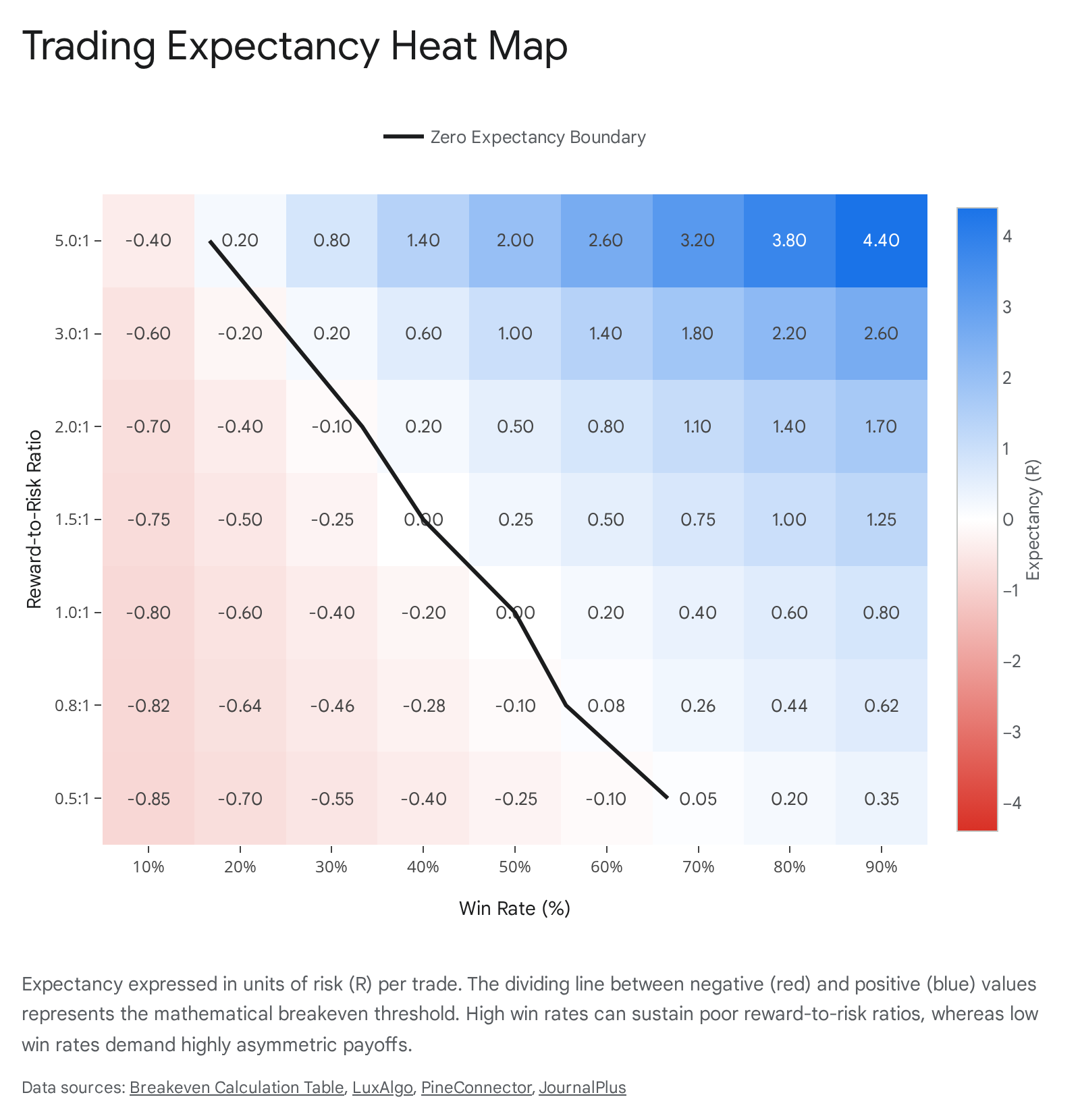
Where $R$ is the reward-to-risk ratio. A positive $E$ signifies a system that generates a net average profit per trade executed, whereas a negative $E$ indicates an inherent mathematical disadvantage 212. The interdependency between the win rate and the reward-to-risk ratio dictates that neither metric possesses standalone analytical value. A 95% win rate holds no structural advantage if the 5% of losses are catastrophic enough to yield a negative net expectancy, just as a highly favorable reward-to-risk ratio is meaningless if the win rate falls below the mathematical breakeven point 67.
Win Rate and Reward-to-Risk Dynamics
To quantify the mathematical threshold of a zero-expectancy system, analysts calculate the breakeven win rate. The formula to determine the precise accuracy required to prevent capital erosion at a specific reward-to-risk ratio is:
$$W_{breakeven} = \frac{1}{1 + R}$$
Where $R$ is the reward-to-risk ratio 9. A system maintaining a 1:1 reward-to-risk ratio requires a strict 50% win rate to break even before the frictional costs of commissions and slippage. As the payoff asymmetry increases, the required accuracy drops precipitously.
| Reward-to-Risk Ratio (R) | Required Breakeven Win Rate (%) | Strategic Market Profile |
|---|---|---|
| 0.1:1 | 90.91% | Arbitrage / High-Frequency Market Making |
| 0.5:1 | 66.67% | Scalping / Mean Reversion |
| 1.0:1 | 50.00% | Symmetric Directional Trading |
| 1.5:1 | 40.00% | Swing Trading |
| 2.0:1 | 33.33% | Intermediate Trend Following |
| 3.0:1 | 25.00% | Standard Trend Following |
| 5.0:1 | 16.67% | Long-Term Trend Following |
| 10.0:1 | 9.09% | Out-of-the-Money Option Buying / Tail Risk Hedging |
Table 1: Breakeven Win Rates Across Reward-to-Risk Profiles 234.
Empirical Strategy Profiles
Empirical data across different trading methodologies reveals a robust inverse correlation between the observed win rate and the reward-to-risk ratio. High-frequency trading (HFT) and market-making strategies typically exhibit high win rates - often exceeding 70% - coupled with low reward-to-risk ratios 25. These strategies capitalize on capturing the bid-ask spread and providing liquidity, taking minimal directional risk and actively managing overnight inventory variance. Regulatory analyses of HFT in futures markets demonstrate that while aggressive firms dominate trading volume and consistently display annualized Sharpe ratios exceeding 9.0, their intraday distribution of returns features massive variance, indicating a reliance on rapid execution of marginal mathematical edges rather than absolute accuracy 6.
Conversely, systematic trend-following Commodity Trading Advisors (CTAs) historically operate with win rates ranging between 20% and 40%, relying on large, infrequent asymmetric payoffs - often exceeding a 3:1 reward-to-risk ratio - to achieve long-term capital growth 647. The objective of trend-following CTAs is to identify medium to long-term trends systematically across diverse asset classes. Because trends are statistically infrequent, these models incur many small losses, resulting in low accuracy but substantial positive expectancy when outliers are captured 78. Benchmark metrics, such as the SG Trend Index and the Barclay BTOP50 Index, track these systematic allocations. Performance data demonstrates that while these strategies can suffer prolonged drawdowns during regime shifts or correlation breakdowns, their underlying mathematical expectancy remains positive due to the magnitude of the right-tail events they capture 816.
Position Sizing and the Mathematics of Ruin
While a positive expectancy theoretically guarantees profitability over an infinite sample size, trading occurs within strict finite constraints of time and capital. A strategy boasting a highly positive expectancy can still result in total capital exhaustion if position sizing is improperly calibrated to the variance of the strategy's return distribution. The calculation of this hazard is known as the "Risk of Ruin."
Fixed-Fractional Sizing and Ruin Probability
Risk of ruin formulas quantify the exact probability that an account will breach a catastrophic drawdown threshold before reaching an intended profit target 11718. This metric highlights the supremacy of position sizing over pure strategy accuracy. One widely utilized derivation, formalized by Perry Kaufman, estimates the risk of ruin for fixed-fractional betting:
$$\text{RoR} = \left( \frac{1 - A}{1 + A} \right)^N$$
Where $A$ is the per-trade edge (expectancy expressed as a fraction of the unit risked), and $N$ represents the total number of risk units in the account (total capital divided by the dollar amount risked per trade) 117.
The formula underscores a fundamental reality of quantitative risk management: if a trading system has zero or negative expectancy ($A \le 0$), the ratio $(1 - A) / (1 + A)$ becomes $\ge 1$. Consequently, raising this ratio to any power yields 1, signifying that the risk of ruin is strictly 100% regardless of how small the initial position size is 1. Position sizing cannot salvage a system lacking a statistical edge.
For a positive-expectancy system, the probability of ruin decays exponentially as $N$ (the number of risk units) increases. For example, a system with a 55% win rate and a 1:1 reward-to-risk ratio holds a positive per-trade edge. If a trader risks 5% of their capital per trade, they possess only 20 risk units ($N=20$), generating a ruin probability in excess of 40% 118. If the same trader reduces the risk to 2% per trade ($N=50$), the probability of ruin drops dramatically, and at 1% risk ($N=100$), it approaches a negligible boundary 118.
| Risk Per Trade | Total Risk Units ($N$) | Win Rate ($W$) | Ruin Probability (Approx.) |
|---|---|---|---|
| 10% | 10 | 55% | 13.50% |
| 5% | 20 | 55% | 1.80% |
| 2% | 50 | 55% | < 0.10% |
| 10% | 10 | 50% (Zero Edge) | 100.00% |
Table 2: Impact of Position Sizing on Ruin Probability for a Constant Edge 118.
Ralph Vince's Optimal Fraction and Leverage Space
Further sophistication in position sizing was introduced by mathematician Ralph Vince through the concept of "Optimal $f$." Vince's models calculate the specific fraction of capital to risk on each independent trade that mathematically maximizes the geometric growth rate of the portfolio over a defined horizon 20.
Plotting expected geometric growth against varying position sizing fractions creates a "leverage space curve." This mathematical surface is deeply asymmetrical. Below the Optimal $f$ peak, the account is under-leveraged, and growth is suboptimal. Exactly at the peak, geometric growth is maximized, but the volatility and drawdowns experienced to achieve this growth are extraordinarily violent, frequently reaching drawdowns in excess of 80% 20. Most critically, sizing above the Optimal $f$ peak leads to a rapid deceleration in growth and inevitable mathematical ruin, even with a highly profitable underlying edge 20.
The practical limitations of theoretical mathematics in trading were demonstrated in an experiment conducted by Vince involving forty doctorates with no background in statistics or trading. Given a simulated environment with a robust 60% win rate and 1:1 payout - a highly positive expectancy - 95% of the participants lost money over 100 trials 9. The failure was entirely attributable to erratic position sizing and the psychological inability to endure variance, resulting in eventual capital depletion despite a persistent mathematical edge 9.
Payoff Asymmetry and Sequential Risk
When evaluating strategies with highly asymmetric payoffs - such as long-volatility tail-risk hedging or early-stage venture capital allocations - classical ruin formulas behave counterintuitively. In these environments, losses are extremely frequent but strictly limited, while gains are rare but massive 1023.
Mathematical models of asymmetric stopping problems reveal that increasing payoff asymmetry (higher potential rewards coupled with lower probabilities of success) can actually increase the likelihood of ruin in positive-return scenarios 1023. The escalated variance increases the probability of exhausting capital through consecutive minor losses before the rare, massive payout occurs to replenish the account. Conversely, for strategies with a net-negative expected return, high payoff asymmetry actually mitigates the immediate probability of ruin compared to a symmetric negative-return game, as a single outlier event can abruptly delay terminal ruin 1023.
Behavioral Distortions in Probability Assessment
Despite the rigid mathematics governing expectancy and risk, human decision-making frequently introduces errors through cognitive biases regarding probability. In market environments, the most pervasive and destructive of these is the Gambler's Fallacy.
Cognitive Mechanisms of the Gambler's Fallacy
The Gambler's Fallacy, conceptually linked to the "Law of Small Numbers," is the erroneous psychological belief that past events influence the probabilities of future independent events in a random or stochastic process 242511. It manifests as the expectation that a short sequence of outcomes must rapidly balance out to reflect the long-term underlying probability distribution 2511.
In trading, this fallacy profoundly distorts the execution of a defined expectancy model. Traders experiencing a cluster of losses in a system may falsely conclude that a winning trade is statistically "due," attempting to impose global randomness onto local sequences 2412. Psychological studies indicate that the Gambler's Fallacy may be rooted in an evolutionary "world model" that expects the rapid replenishment of natural resources, a heuristic that fails completely in modern financial environments 12.
This heuristic failure induces several mathematically ruinous behaviors: 1. Averaging Down: Increasing exposure to a losing position under the assumption that a mean-reverting bounce is statistically overdue, thereby compounding negative expectancy 24. 2. Over-leveraging Post-Drawdown: Expanding position sizes after a losing streak to quickly recoup losses, under the false assumption that the probability of the next trade being a winner has sequentially increased 24. 3. Chasing Reversals: Entering counter-trend positions prematurely simply because a trend has persisted longer than intuitive expectations allow, ignoring the empirical reality of heavy-tailed market distributions 2412.
The Impact of Negative Autocorrelation in Decision Making
Research spanning diverse decision-making domains confirms the prevalence of this bias. Studies analyzing judicial rulings, loan approvals, and financial market decisions reveal that humans actively exhibit negatively autocorrelated choices - meaning they force an alternation of decisions if they perceive a streak occurring - simply to align with their internal representation of fairness or randomness 1128.
For systematic trend followers, whose systems possess win rates below 40%, long streaks of continuous losses are mathematically expected. A failure to endure these normal streaks, driven by the psychological pressure of the Gambler's Fallacy, results in system abandonment just before the low-probability, high-magnitude outlier trend materializes 724.
Autocorrelation and the Sequence of Returns
The classic calculation of risk of ruin assumes that trade outcomes are perfectly independent, identically distributed (i.i.d.) random variables. However, financial markets are not frictionless environments; asset returns, and by extension trading system equity curves, frequently exhibit serial correlation (autocorrelation). The presence of autocorrelation fundamentally alters the actual expectancy and survival probability of a trading edge.
Serial Correlation in Price Dynamics
Serial correlation measures the degree to which a variable's current value is related to its past values over a specific time lag 131415. If asset returns exhibit positive autocorrelation, trends are likely to persist (momentum); if they exhibit negative autocorrelation, price movements are likely to reverse (mean reversion) 131415.
Historically, researchers have found varying levels of autocorrelation depending on the time horizon and market context. Intraday and daily returns of large-cap equities often exhibit negative serial correlation 1633. Theoretical models, such as those established by Campbell, Grossman, and Wang (1993), suggest this negative first-order daily autocorrelation is heavily driven by trading volume 17. When noninformational "liquidity" traders demand sudden execution, risk-averse market makers accommodate the order flow but extract a premium by altering the stock price. This leads to an expected reversal the following day to reward the market maker for providing liquidity 1718. Consequently, price declines accompanied by abnormally high volume have a mathematically higher probability of reversing, resulting in reduced autocorrelation on high-volume days 17.
Trade Sequence Dependency and the Z-Score
When the underlying assets exhibit autocorrelation, the trading strategies applied to them generate equity curves that are also autocorrelated. To test whether the sequence of wins and losses is truly independent, quantitative analysts utilize the Z-score metric for dependence:
$$Z = \frac{N(R - 0.5) - P}{\sqrt{\frac{P(P - N)}{N - 1}}}$$
Where $N$ is the total number of trades, $R$ is the total number of streaks (runs), and $P = 2 \times W \times L$ (with $W$ and $L$ representing the total count of winning and losing trades) 3637.
A Z-score near zero indicates that trades are entirely independent. A Z-score greater than +2.0 indicates a statistically significant negative dependency (profits and losses alternate frequently), while a Z-score below -2.0 indicates a positive dependency (profits and losses cluster into heavy streaks) 361920.
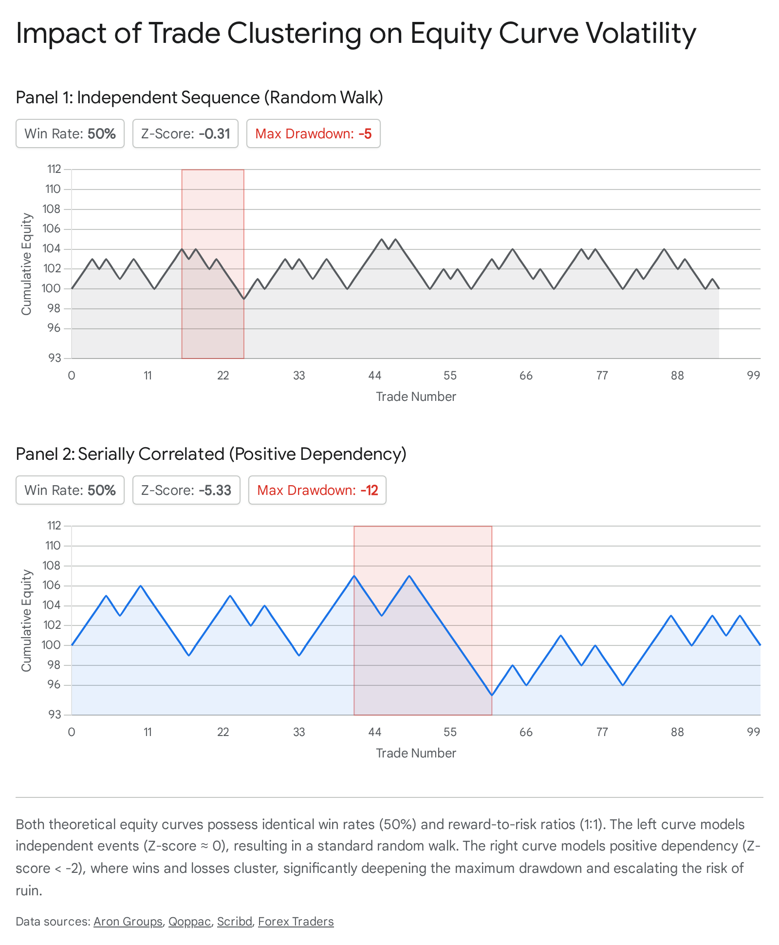
Trend-following systems generally exhibit negative Z-scores; because trends are rare, losses cluster tightly together during range-bound sideways markets, invalidating the assumption of independent events used in basic mathematical ruin models 361940.
The presence of serial correlation mandates adjustments to position sizing. If an equity curve exhibits positive autocorrelation (losing trades cluster together), the actual risk of ruin is substantially higher than the theoretical calculation 3640.
Market Regimes and Structural Non-Stationarity
Market autocorrelation is not static; it fluctuates as the market shifts through distinct macroeconomic or structural phases known as "regimes" (e.g., low-volatility bull markets transitioning to high-volatility bear markets) 214222. Because trading systems are optimized for specific market environments, a system that exhibits positive expectancy in one regime may experience rapid edge degradation when the regime shifts abruptly.
Markov Switching and Latent State Detection
To detect these unobservable shifts, quantitative researchers utilize Hidden Markov Models (HMM) and Gaussian Mixture Models (GMM) 222324. An HMM assumes that the market is driven by a finite set of unobserved (latent) states. Each state emits observable data - such as specific means, variances, and cross-asset correlations - according to its own probability distribution 4224.
Crucially, transitions between these states are governed by a Markov transition matrix, which quantifies the exact probability of the market remaining in its current regime versus switching to another. For example, a transition matrix might indicate a 97.75% probability of remaining in a low-volatility state day-over-day, but a 4.53% probability of transitioning to a high-volatility regime 4224.
By modeling regimes mathematically, portfolio managers can adjust their conditional expectancy expectations. Ang and Timmermann established that ignoring regime changes carries a substantial economic cost; the risk-return trade-offs are highly non-linear across different states, with skewness and fat tails expanding significantly during persistent bear regimes 21. Dynamic position sizing, dictated by the output of a Hidden Markov Model, allows allocators to shift capital away from strategies that mismatch the current latent state before catastrophic drawdowns accumulate 212324.
Market Microstructure and Execution Friction
Edge degradation and ruin probability are heavily influenced by exogenous execution factors, primarily slippage, transaction costs, and market impact. A positive theoretical expectancy on paper can immediately turn negative in live execution if the market cannot absorb the order efficiently.
Asymmetric Liquidity and Hidden Orders
Institutional trading impact is rarely linear. Research into the incremental execution of large orders demonstrates that the presence of heavy-tailed order sizes leads to persistence in the signs of transactions - buyer-initiated trades tend to cluster with other buyer-initiated trades 25. This predictability in order flow implies that to preserve market efficiency, liquidity must become asymmetric. The market impact of executing a large order becomes a concave function of the order size, deteriorating the entry price and directly eroding the reward-to-risk ratio 25. If market impact increases rapidly with volume, a fund's size is severely constrained, potentially turning a profitable backtested strategy into a losing live strategy 25.
Trade Clustering and Systemic Ruin Vulnerability
The proliferation of algorithmic trading has led to "market clustering," a phenomenon where a significant portion of market participants execute highly correlated strategies based on shared signals 262728. Research utilizing bipartite network representations of granular equity trading data demonstrates that an increase in market clustering directly reduces the diversity of the investor pool 2627.
When heterogeneous actors simultaneously act on similar momentum or mean-reversion metrics, coincidental overlap transforms into "crowded trades" 2629. This homogeneity strips liquidity from the market precisely when participants require it to exit positions simultaneously, resulting in heightened price instability and heavier tails in the return distribution 2628. In highly clustered markets, a trader's genuine risk of ruin is elevated far beyond the strategy's theoretical backtest parameters, as slippage and impact costs exponentially increase during crowded exit events 2627.
Statistical Validation and Backtest Overfitting
The calculations of expectancy, reward-to-risk, and optimal position sizing are entirely dependent on the assumption that the historical parameters of a trading strategy will persist into the future. In quantitative finance, establishing this premise relies on rigorous backtesting. However, modern computational power has facilitated a crisis of reproducibility through backtest overfitting and data mining 513031.
Sample Size Constraints and Statistical Power
A trading edge is only valid if it is statistically significant - meaning the likelihood that the observed returns were generated by random chance is sufficiently low. To evaluate significance, analysts utilize p-values, t-tests, and the Sharpe ratio, but these metrics are acutely sensitive to sample size 54.
Statistically, a minimum threshold of approximately 30 independent trades is required to rely on the Central Limit Theorem to approximate a normal distribution of sample means, though modern practitioners demand significantly more (often >100 to 1,000 trades) to reliably estimate expectancy and variance 154. Furthermore, these trades must be truly independent; a high-frequency strategy executing 500 trades during a single highly autocorrelated trending period possesses a much lower effective sample size than a strategy generating 50 independent trades across diverse macroeconomic volatility regimes spanning a decade 54.
P-Hacking and the False Strategy Theorem
"P-hacking" in finance refers to the exploitation of undisclosed flexibility in data analysis to hunt for statistical significance ($p \le 0.05$) 3032. With granular financial data, researchers can manipulate independent variables, alter lookback windows, apply different outlier exclusion rules, and transform series data until a seemingly highly profitable trading rule emerges 3032.
This generates severe backtest overfitting. As formulated in the False Strategy Theorem (Bailey et al.), if an analyst evaluates a sufficiently large number of strategy parameter variations on a single historical dataset, the probability of finding a variant that appears highly profitable - even if the underlying data is a pure random walk - approaches absolute certainty 5131. For example, quantitative studies indicate that after computing just 1,000 variations of a strategy on entirely random data, the expected maximum Sharpe ratio of the "optimal" fit can easily exceed 3.0, purely as a mathematical artifact of selection bias under multiple testing 5131. Consequently, strategies possessing brilliant historical equity curves frequently fail entirely out-of-sample, directly eroding investor capital 3133.
Protocols for Robust System Evaluation
To combat edge degradation via overfitting, quantitative finance researchers, notably Campbell Harvey, have advocated for drastically higher thresholds for statistical significance. Following an exhaustive evaluation of over two million trading strategies and documented anomalies across global stock markets, Harvey et al. determined that the traditional $t$-statistic threshold of 2.0 ($p=0.05$) is entirely inadequate due to the sheer volume of multiple testing occurring industry-wide 343536. They argue for significantly higher hurdles, such as a minimum $t$-statistic of 3.0, to declare a financial anomaly or trading signal robust 35.
Practitioners implement several robust machine-learning-inspired protocols to validate true expectancy and survive live execution: * Out-of-Sample Holdouts: Strictly dividing historical data into training (in-sample) and testing (out-of-sample) sets, ensuring the optimal parameters are never exposed to the test data until the final performance evaluation 3133. * Dimensionality Reduction: Employing techniques such as random subspace or stepwise regression to limit the number of predictive variables, penalizing model complexity to prevent the algorithm from memorizing historical noise 6061. * Data Aggregation: Enhancing statistical power by testing identical model parameters across a broad cross-section of unrelated instruments (e.g., applying the exact same momentum threshold to 3,000 distinct equities concurrently rather than optimizing individually per stock) to eliminate idiosyncratic curve-fitting 6061. * Walk-Forward Analysis and Bootstrapping: Utilizing resampling techniques (sampling with replacement) to simulate thousands of alternative equity paths. By analyzing the 5th percentile of these Monte Carlo simulations, traders can estimate a much more accurate, stress-tested maximum drawdown and adjust their empirical risk of ruin calculations accordingly before committing live capital 5462.
Ultimately, the survival of a trading edge is not determined merely by its raw historical win rate or reward-to-risk ratio. It is dictated by a multifaceted mathematical framework that demands rigorous statistical validation, precise ruin probability modeling, active awareness of structural autocorrelation and regime transitions, and disciplined position sizing designed to withstand the inevitable friction of complex financial ecosystems.