Sparse mixture-of-experts models and efficiency
Introduction to Sparse Neural Networks
The evolution of artificial intelligence over the past decade has been heavily defined by scaling laws, which dictate that increasing the parameter count of a neural network and the volume of its training data yields predictable, proportional improvements in model capabilities. This paradigm reached a critical inflection point with the advent of massive dense architectures, establishing a baseline for natural language processing that dominated the early 2020s. However, the trajectory of dense scaling has encountered severe physical and economic barriers. As organizations push toward trillion-parameter milestones, the computational cost, power consumption, and hardware requirements of monolithic dense networks have become increasingly unsustainable. The necessity to process every single parameter for every token of input data creates a computational bottleneck that threatens to halt the rapid advancement of artificial general intelligence.
In response to these limitations, the machine learning industry has widely adopted Mixture-of-Experts architectures. Initially conceptualized in 1991, this methodology has been modernized to serve as the foundation of the contemporary efficiency frontier in large language models. The architecture operates on the principle of conditional computation, decoupling a model's total parameter count from its active computational cost. By partitioning the network into specialized sub-networks and employing dynamic routing mechanisms, a sparse model selectively activates only a fraction of its total parameters for any given input. This enables the model to store a vastly larger repository of knowledge than a compute-equivalent dense model while operating with significantly reduced latency and computational overhead.
The transition to sparse models represents a structural shift that is fundamentally reshaping the deployment landscape of artificial intelligence. By late 2025 and early 2026, the majority of frontier model releases from both proprietary laboratories and open-weights initiatives have integrated these sparse paradigms. This transition necessitates a profound reevaluation of model training dynamics, hardware optimization, and network load balancing, as the primary constraints of model design shift from raw floating-point operations to memory bandwidth and interconnect communication latency.
The Dense Scaling Bottleneck
To understand the necessity of sparse architectures, one must first examine the mathematical and hardware limitations of dense networks. In a dense large language model, every parameter within the network is activated for every single input token during both the forward and backward passes. This structural rigidity ensures robust learning but introduces immense computational inefficiencies at scale.
The GPT-3 architecture serves as the archetypal example of the dense scaling paradigm. Released in 2020, the 175-billion-parameter variant of GPT-3 demonstrated that language models could achieve strong few-shot learning capabilities entirely through scale. The architecture consists of a dense decoder-only transformer with 96 attention layers, a hidden dimension of 12,288, and 96 attention heads 123. During a forward pass, processing a single token requires the activation of all 175 billion parameters. Because the computational complexity of the feed-forward network layers is defined by $O(d_{\text{model}} \times d_{\text{ff}})$, generating a single token requires approximately 350 billion multiply-add operations 3.
As model sizes expand beyond the 100-billion-parameter threshold, the brute-force computational cost becomes prohibitive. Training dense models requires advanced distributed training techniques, including tensor parallelism, pipeline parallelism, and data parallelism, to partition the model across thousands of graphics processing units 15. The energy demands of such clusters are staggering; training a massive dense model can consume tens of megawatts of power, with future infrastructure build-outs projecting power requirements in the gigawatt range 4. Furthermore, inference becomes highly inefficient. Paying the computational cost of the entire network for every token regardless of the token's complexity - allocating the same computational resources to process a simple punctuation mark as a complex mathematical eigenvalue - wastes hardware capacity 3. This inefficiency is the primary catalyst for the widespread adoption of conditional computation.
Structural Foundations of Mixture-of-Experts
The core innovation of the modern sparse architecture in transformer-based language models lies in the replacement of standard dense feed-forward network layers with sparsely activated expert layers.
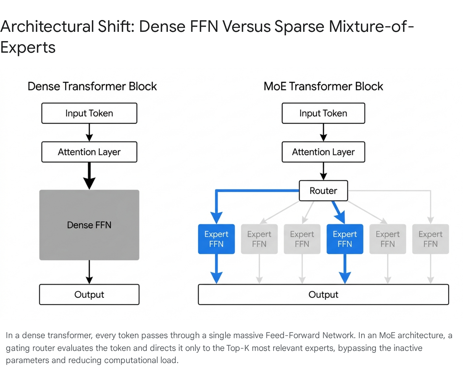
In a standard transformer block, the feed-forward network is a monolithic structure that applies the same weight matrices to every token in the sequence 3. The transformer architecture typically allocates roughly seventy to eighty percent of its total parameter count to these feed-forward blocks, making them the most logical target for architectural modification 56.
In a sparsely activated layer, this single feed-forward network is replaced by a set of $E$ distinct expert networks. Each expert operates as an independently parameterized multi-layer perceptron, possessing its own unique weight matrices 37. The decision regarding which expert processes which token is governed by an auxiliary gating network, commonly referred to as a router.
For a given input token sequence, the router computes a probability distribution over the available experts, producing gating weights that determine the relative contribution of each expert to the final output 310. The output of the layer is mathematically defined as the linearly weighted sum of the outputs from the selected experts. Sparsity is explicitly enforced by constraining the gating network such that only $K$ out of the $E$ experts receive non-zero gating weights, a parameter defined as the Top-$K$ routing strategy 311. The unselected experts contribute nothing to the computation for that specific token, meaning their weight matrices are neither loaded from memory nor multiplied 3. By maintaining a constant $K$ while increasing $E$, researchers can dramatically increase the total parameter capacity of the model without proportionally increasing the computational operations required per forward pass 128.
Gating Mechanisms and Routing Algorithms
The theoretical advantages of conditional computation are entirely dependent on the efficiency and stability of the gating network. If the router fails to effectively distribute tokens across the available parameter space, the model will lose the benefits of its specialized capacity. Over the years, several distinct routing algorithms have been developed to address the computational limitations and training instabilities of early sparse network implementations.
Token Choice Routing and Load Imbalance
In traditional sparse architectures, the gating mechanism operates on a paradigm known as Token Choice routing 915. Under this methodology, each individual token independently evaluates the available parameter blocks and selects the top experts that yield the highest affinity scores based on its own criteria 9. The router computes logits by multiplying the input representations by the router weights, applies a softmax normalization, and dispatches the token to the indices with the highest probability 616.
While computationally straightforward, Token Choice routing suffers from a severe systemic flaw: load imbalance 817. Because tokens act independently without global awareness of the batch, the router frequently discovers early in the training process that a small subset of experts is marginally better at handling generic language patterns 18. This initiates a positive feedback loop: the router funnels a disproportionate number of tokens to these popular experts, providing them with more forward pass data and stronger gradient signals during backpropagation 3. As these experts become better trained, the router sends them even more tokens. This phenomenon, known as expert collapse, results in massive computational bottlenecks 3. The overworked experts slow down the entire system, while the remaining experts sit idle, receiving no training signal and stagnating. The model effectively collapses back into a smaller, dense network, wasting the majority of its parameter capacity 18.
To mitigate expert collapse, engineers typically implement strict hardware capacity limits, or buffer constraints, on each individual expert. The capacity is calculated by dividing the total number of tokens by the number of experts and multiplying by a capacity factor 816. If an expert receives tokens exceeding its buffer limit, the excess tokens are summarily dropped and passed to the next layer without undergoing feed-forward processing, which severely degrades output quality 91610. Furthermore, to force the router to utilize all experts, an auxiliary load-balancing loss must be added to the training objective 816. This mathematical penalty forces the router to distribute tokens more evenly, essentially sacrificing optimal token-to-expert affinity simply to ensure hardware utilization 1618. Despite these regularizations, Token Choice systems routinely require overprovisioning expert capacity by massive margins - often two to eight times the calculated requirement - to absorb transient spikes in token distribution, resulting in significant wasted memory and compute 89.
Expert Choice Routing
Recognizing the inherent inefficiencies of independent token selection, researchers at Google introduced the Expert Choice routing mechanism at NeurIPS 2022 to optimize load balancing without relying on destructive auxiliary losses 817. This architectural revision fundamentally inverts the assignment logic: rather than tokens selecting the most appropriate experts, each expert selects the top tokens it is best suited to process from a given sequence batch 915.
In Expert Choice routing, the gating network generates a comprehensive token-to-expert affinity matrix for the entire input sequence. However, instead of applying a top-selection function across the expert dimension for each token, the routing algorithm applies the selection function across the token dimension for each expert 78. Every expert is assigned a strict, predetermined buffer capacity defined by a global capacity factor, which dictates the average number of experts that will process each token 8.
This inversion guarantees perfect load balancing by algorithmic design. Because every expert selects exactly its maximum capacity of tokens, no expert is ever left idle, and no expert is ever overloaded 820. Consequently, it completely eliminates the need for auxiliary load-balancing loss functions, allowing the model to route tokens purely based on affinity 810. An additional architectural consequence of Expert Choice is heterogeneous token routing. Inherently complex or crucial tokens might be selected by multiple experts simultaneously, receiving deeper computational analysis, while simple tokens might be selected by fewer experts, thereby allocating processing power dynamically where it is most needed 8.
Despite its advantages in training convergence, Expert Choice routing introduces complications during autoregressive inference. Because the algorithm requires observing a large batch of input sequences to perform the global top-token selection, it struggles in single-token generation scenarios where the future token pool is nonexistent 10.
Soft Mixture-of-Experts
While both Token Choice and Expert Choice rely on discrete, hard assignments - where a token is definitively routed to an expert or it is not - Soft Mixture-of-Experts introduces a fully differentiable, continuous routing paradigm 9. Standard discrete routing requires solving complex linear assignment problems or using non-differentiable approximations, which can cause training instability and optimization difficulties 2122.
The Soft Mixture-of-Experts algorithm discards the concept of sending a specific token to a specific expert. Instead, the architecture passes different weighted combinations of all tokens to every expert simultaneously 2123. The system computes an affinity matrix between the batch of input tokens and a set of learnable parameter vectors known as "slots" 923. By applying a softmax normalization function over the columns of this matrix, the model generates a set of dispatch weights. These weights combine the input tokens into a precise linear mixture for each slot 212411. Every expert then processes its assigned slots. Following the expert computation, a second softmax normalization is applied across the rows of the original matrix to create combine weights, which distribute the processed slot outputs back to the original token dimensions 2126.
Because the algorithm computes a linear combination of all input tokens for every expert, it completely sidesteps the token dropping problem and eliminates expert imbalance, as every expert is guaranteed to receive a mathematically uniform block of data 923. This fully differentiable approach resolves sequence-level determinism issues and has demonstrated significant success in scaling vision transformers, where it outperforms both discrete sparse architectures and dense networks by maintaining optimal parameter utilization 1112. However, the computational overhead of continuous token mixing imposes heavier limits on video random access memory (VRAM) footprint during inference compared to sparse discrete methods 2313.
Auxiliary-Loss-Free and Alternative Routing
To bridge the gap between the autoregressive compatibility of Token Choice and the load-balancing superiority of Expert Choice, contemporary models have developed auxiliary-loss-free discrete routing mechanisms. Models like DeepSeek-V3 introduce an architectural component where the router dynamically monitors the historical load of each expert. If an expert becomes overburdened, the system automatically adjusts a specialized bias term downward, artificially lowering the expert's affinity scores for subsequent tokens 2914. This technique enforces strict load balancing across hundreds of experts without incorporating a separate loss function that penalizes the primary training objective 2914.
Other alternative gating mechanisms have also been deployed in specialized environments. Hash-based routing abandons learned affinity altogether, using deterministic hashing algorithms to route tokens, which removes the parameter overhead of the gating network entirely 6. Noisy Top-K routing, utilized in earlier sparsely gated networks, injects tunable Gaussian noise into the logits before selection, artificially increasing exploration and preventing the router from collapsing into repetitive assignment patterns early in the training phase 626.
| Routing Algorithm | Selection Mechanism | Load Balancing Strategy | Inference Complexity | Primary Drawback |
|---|---|---|---|---|
| Token Choice | Tokens select the Top-$K$ experts 9. | Relies on auxiliary loss and strict buffer limits 816. | Highly efficient for autoregressive step-by-step generation. | Prone to token dropping, expert collapse, and capacity waste 38. |
| Expert Choice | Experts select the Top-$K$ tokens 8. | Perfect structural balance; experts fill fixed capacities 10. | Difficult to implement in small-batch autoregressive decoding 10. | Requires full batch context prior to assignment 1012. |
| Soft Assignment | Continuous weighted matrix multiplication 11. | Implicitly balanced; all experts process token mixtures 923. | High overhead due to dense matrix mixing at every step 23. | Increases memory bandwidth constraints during token mixing 23. |
| Auxiliary-Loss-Free | Tokens select experts with dynamic bias penalties 29. | Algorithmic bias term adjustments based on real-time load 14. | Highly efficient, native autoregressive compatibility 14. | Requires precise tuning of bias adjustment hyper-parameters. |
Granularity and the Shared Expert Paradigm
A persistent architectural flaw in standard sparse networks is the phenomenon of knowledge redundancy. In a traditional configuration utilizing eight distinct experts, all eight sub-networks must individually dedicate a portion of their parameter capacity to learning basic, high-frequency elements of the training data, such as basic grammar, punctuation handling, and universal syntax 318. This widespread duplication wastes valuable parameter real estate that could otherwise be dedicated to deep specialization.
To eliminate this redundancy, advanced architectures have pioneered the Shared Expert paradigm. This structural evolution separates the network into two distinct pools: a large set of fine-grained routed experts and a smaller set of permanently activated shared experts 2931. The shared experts are isolated from the dynamic routing mechanism and are structurally forced to activate for every single token passing through the layer. They act as the repository for universal foundational knowledge and baseline transformations 2915.
By offloading the processing of common language mechanics to the shared experts, the dynamically routed experts are freed to become highly specialized in niche domains, capturing potentially non-overlapping subsets of the model's knowledge 2931. This isolation drastically reduces redundancy. Furthermore, to maximize the combinatorial diversity of the ensemble, the dynamically routed experts are subject to fine-grained segmentation. Instead of utilizing a small number of large experts, the parameter space is divided into a massive array of smaller experts - for instance, replacing 8 massive feed-forward networks with 256 much smaller ones 293133. Despite this exponential increase in expert count, the overall parameter activation per token remains constrained, resulting in richer representational capacity without incurring additional computational penalties 2931.
Hardware Constraints and System Infrastructure
The transition from dense to sparse architectures fundamentally alters the hardware bottlenecks encountered during model training and deployment. While conditional computation successfully decouples theoretical parameter capacity from raw floating-point operations, it introduces severe constraints on memory bandwidth and network interconnects, reshaping how data centers must be designed.
The Memory Bandwidth Bottleneck
Dense language models are typically constrained by compute limits; because every parameter is used to process every token, the primary bottleneck is the speed at which the graphics processing unit's arithmetic logic units can execute matrix multiplications 318. In stark contrast, sparse architectures are almost exclusively memory-bound, particularly during autoregressive inference 1834.
During generation, a sparse model may only activate a minute fraction of its parameters - sometimes as low as two to five percent. However, because the router dynamically selects experts on a per-token basis, the system cannot predict which specific experts will be required for the next token in the sequence. Consequently, the entirety of the model's weight matrices must remain continuously loaded in the physical Video RAM (VRAM) of the hardware array 1813. For example, while a model with 141 billion parameters may operate with the computational latency of a much smaller network, it still requires the massive VRAM footprint to house all 141 billion parameters across multiple devices 35. The operational bottleneck shifts entirely from executing arithmetic to shuttling massive weight matrices from the high-bandwidth memory to the processor cores. If the hardware and software are not explicitly optimized for these sparse, unpredictable memory access patterns, cache misses and memory transfer latency can negate the theoretical speed advantages of the architecture 1834.
Distributed Training and Expert Parallelism
Because state-of-the-art sparse models contain hundreds of billions - or even trillions - of parameters, their memory footprint vastly exceeds the capacity of any single computational accelerator. They require distributed multi-node clusters, introducing a requirement for Expert Parallelism 612. In an expert-parallel deployment, different physical devices host different subsets of the expert networks 6.
In a dense model, data exchange between processors follows a highly predictable, choreographed routine dictated by standard pipeline and tensor parallelism, allowing network engineers to tune cluster communications to near-maximum efficiency 3616. In a sparse model, routing is improvisational and stochastic, determined entirely at runtime by the input data 736. When a token processed on one device is routed to an expert residing on a different device, the token must be transmitted across the physical network interconnect. This architecture triggers a massive, unpredictable All-to-All communication step at every single sparse layer in the network 71216. Every device must send tokens to, and receive outputs from, multiple other devices simultaneously.
As a result, the physical network interconnects - such as specific configurations of InfiniBand or custom high-speed fabrics - become the primary bottleneck for scaling. Communication overhead from expert-routing traffic can account for a substantial percentage of total per-token latency in production environments, making interconnect bandwidth more critical than raw compute performance when designing infrastructure for sparse networks 1236.
Inference Optimization and Offloading
To mitigate the massive memory requirements of sparse networks, engineering teams deploy an array of inference optimization strategies. When deploying extremely large models on resource-constrained infrastructure, developers frequently utilize offloading techniques. Inactive expert parameters are housed in standard system RAM or fast NVMe solid-state drives, and are dynamically swapped into the GPU's VRAM only when the routing mechanism calls for them 6. While this enables massive models to run on consumer-grade hardware, the bandwidth limitations of the PCIe bus introduce severe latency penalties, significantly reducing token generation speeds 3438.
To optimize memory pathways on enterprise clusters, developers leverage extremely localized gating algorithms, cache highly probable expert paths, and compress the model weights using INT4 or FP8 quantization protocols 133517. These compression techniques drastically reduce the physical size of the expert matrices, allowing more parameters to fit within a single node and minimizing the necessity for cross-node All-to-All communications 3516.
Architectural Analysis of Frontier Models
The commercial and open-weights artificial intelligence ecosystem is now dominated by variations of the sparse architecture. A detailed structural analysis of the leading models reveals how theoretical routing concepts are implemented at the absolute limits of scale.
The GPT-4 Paradigm Shift
While OpenAI maintains stringent secrecy regarding the precise technical specifications of the GPT-4 architecture, widespread industry consensus and research analysis indicate that it relies on a massive sparse framework 401819. The system reportedly marks a significant architectural departure from its dense predecessor, GPT-3, which utilized 175 billion parameters.
GPT-4 is estimated to contain approximately 1.76 to 1.8 trillion total parameters, distributed across 120 layers of neural network 401820. The architecture reportedly employs an ensemble of 16 distinct experts within its feed-forward layers, with each expert containing roughly 111 billion parameters 4044. The model utilizes a straightforward Token Choice Top-2 routing algorithm, meaning each individual token is evaluated and dispatched to the two most relevant experts per forward pass 40.
Coupled with approximately 55 billion shared parameters dedicated to global self-attention mechanisms, the active parameter count during the generation of a single token is constrained to roughly 280 billion 40. By operating as a sparse network, GPT-4 achieves vastly improved inference economics. Generating a forward pass on a dense model of equivalent scale would demand an impractical 3,700 TFLOPs of compute; the sparse implementation requires only approximately 560 TFLOPs 40. The model was trained on an expansive corpus of approximately 13 trillion tokens over multiple epochs, necessitating a distributed cluster of thousands of GPUs operating in complex tensor and pipeline parallel configurations 4021.
The Mixtral Open-Weights Architecture
Mistral AI catalyzed the integration of sparse networks into the open-weights community with the release of the Mixtral model family, empirically proving that relatively small sparse models could outperform massive dense architectures while executing inference at significantly faster speeds 2247.
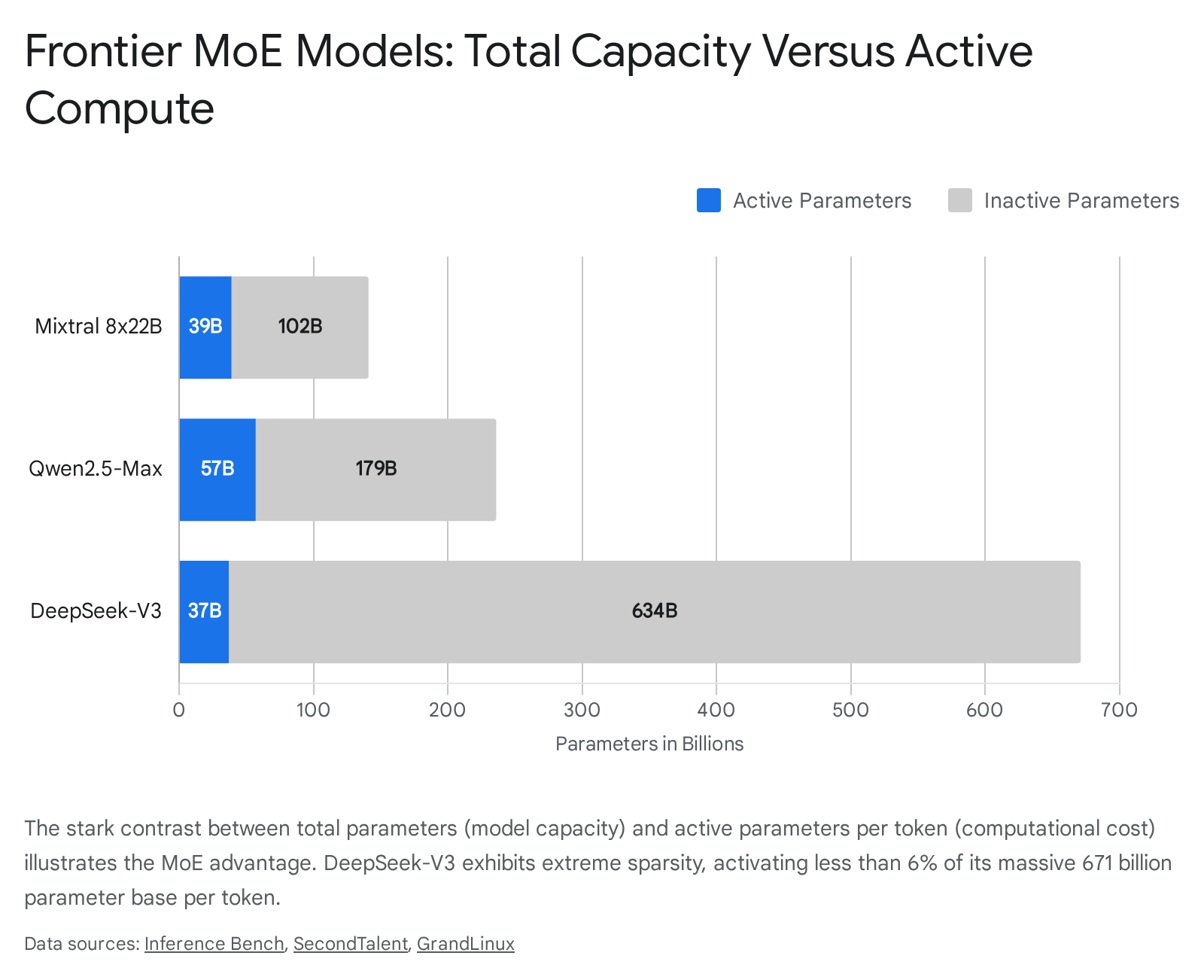
The flagship model of this series, Mixtral 8x22B, consists of 141 billion total parameters distributed across 56 decoder layers 3548. At each layer, the architecture utilizes 8 distinct feed-forward experts. The network employs a Top-2 routing mechanism, dynamically selecting two experts to process each token 63848. Consequently, despite the massive 141-billion-parameter storage footprint, only 39 billion parameters are actively engaged per token 3548. This highly selective activation allows the model to process data at the computational cost of a dense 40-billion-parameter model 3822. The model architecture utilizes Grouped-Query Attention to manage context windows up to 65,536 tokens, ensuring memory efficiency during long-form generation tasks 35.
DeepSeek-V3 and Extreme Sparsity
DeepSeek-V3 represents one of the most sophisticated and highly optimized iterations of the sparse paradigm to date, aggressively pushing the boundaries of both training efficiency and architectural complexity. The model boasts a staggering 671 billion total parameters but achieves extreme sparsity by activating only 37 billion parameters per token - representing an activation rate of less than 6% 34950.
The architecture abandons the standard configuration of a small number of massive experts in favor of ultra-fine-grained segmentation. DeepSeek-V3 distributes its capacity across 256 dynamically routed experts alongside one dedicated shared expert that permanently processes every token to capture universal syntax and foundational knowledge 293350. The routing network employs a Top-8 selection algorithm from the pool of 256 routed experts 33.
To mitigate the severe memory bandwidth bottlenecks inherent in sparse inference, the developers engineered a novel Multi-Head Latent Attention mechanism. This innovation compresses the Key-Value cache via low-rank latent projections, reducing the memory footprint by a factor of 57 compared to standard multi-head attention 201434. This massive reduction in cache size frees up critical memory bandwidth to stream the dense MoE weight matrices during autoregressive generation. Furthermore, the model utilizes an auxiliary-loss-free load balancing strategy, dynamically updating a bias term for each expert based on historical load to prevent expert collapse without sacrificing token affinity 2914. Through these architectural optimizations and the implementation of FP8 precision training, DeepSeek-V3 required only 2.788 million H800 GPU hours to train on a 14.8-trillion-token dataset 201449.
Qwen2.5-Max and the 236-Billion-Parameter Scale
Alibaba Cloud's Qwen2.5-Max is a top-tier proprietary sparse model introduced to compete directly with models like DeepSeek-V3 and GPT-4. While the organization maintains closed weights, technical disclosures indicate the model possesses a total capacity of approximately 236 billion parameters, activating 57 billion parameters per token 5152.
The architecture relies on a 64-expert routing framework, activating 8 experts per token dynamically via its gating network 5153. The model was pre-trained on an extensive multilingual corpus exceeding 20 trillion tokens, encompassing academic papers, code repositories, and diverse web data 5253. By aggressively restricting the active compute to 57 billion parameters, the architecture achieves inference latencies up to 40% faster than dense models of equivalent analytical performance deployed on identical hardware arrays 51. The model explicitly targets benchmark superiority in complex reasoning, coding, and mathematical analysis, incorporating deep reinforcement learning from human feedback protocols into its post-training pipeline 5253.
The Efficiency Frontier: Dense Versus Sparse Models
To objectively quantify the efficiency frontier established by sparse architectures, their structural economics must be benchmarked directly against the pinnacle of contemporary dense network design. Meta's Llama 3.1 405B currently serves as the definitive flagship for dense architectures.
Llama 3.1 405B is an optimized, dense, decoder-only transformer. The architecture consists of 126 layers, 128 attention heads, and a massive hidden dimension of 16,384 355423. Because it is a fundamentally dense model, every single one of its 405 billion parameters is fully active during both the forward and backward training passes, as well as during generation inference 4954. The brute-force nature of this continuous density requires overwhelming computational resources. Training the Llama 3.1 405B variant on a 15.6-trillion-token corpus necessitated approximately 30.8 million H100 GPU hours, monopolizing a dedicated cluster of up to 16,000 top-tier graphics processors 4954. The financial burden of this training run is estimated to be between $92.4 million and $123.2 million 49. Furthermore, serving a 405-billion-parameter dense model in production is exceptionally arduous, requiring advanced multi-node pipeline and tensor parallelism techniques simply to distribute the compute load across multiple server racks 16.
When contrasting this dense paradigm against DeepSeek-V3, the economic and operational divergence of the two architectural philosophies becomes unmistakable. Both models were trained on remarkably similar data volumes - 15.6 trillion tokens for Llama 3.1, and 14.8 trillion tokens for DeepSeek-V3 - and both models achieve highly comparable state-of-the-art results across complex reasoning, coding, and mathematical benchmarks 144924.
However, DeepSeek-V3's heavily optimized sparse architecture required only 2.788 million GPU hours to train - an order of magnitude less computational time than Llama 3.1 405B 201449. By relying on fine-grained expert segmentation and activating only 37 billion parameters per token, DeepSeek fundamentally lowered the per-step mathematical operations required without sacrificing the aggregate storage capacity of the network 49. Consequently, DeepSeek-V3 achieved a training cost per trillion tokens of approximately $378,000, compared to Llama 3.1's estimated $5.93 million to $7.90 million per trillion tokens 49.
This stark contrast perfectly illustrates the efficiency frontier. Sparse conditional computation allows organizations to decouple the theoretical intelligence plateau of a model from exponential compute budgets, maximizing analytical performance relative to the floating-point operations consumed 1257.
| Architectural Specification | Meta Llama 3.1 405B | DeepSeek-V3 | Mixtral 8x22B | Qwen2.5-Max |
|---|---|---|---|---|
| Architecture Type | Dense | Sparse (DeepSeekMoE) | Sparse (SMoE) | Sparse (MoE) |
| Total Parameter Count | 405 Billion 54 | 671 Billion 50 | 141 Billion 35 | ~236 Billion 51 |
| Active Params / Token | 405 Billion 35 | 37 Billion 50 | 39 Billion 35 | ~57 Billion 51 |
| Expert Distribution | N/A (Dense) | 256 Routed + 1 Shared 33 | 8 Routed 48 | 64 Routed 53 |
| Routing Algorithm | N/A (Dense) | Top-8 (Aux-Loss-Free) 714 | Top-2 48 | Top-8 51 |
| Context Window Limit | 131,072 Tokens 35 | 131,072 Tokens (Max 160K) 3525 | 65,536 Tokens 35 | 128,000 Tokens 26 |
| Transformer Layers | 126 Layers 23 | 61 Layers 50 | 56 Layers 35 | Undisclosed |
| Estimated Training Cost | ~$92M - $123M 49 | ~$5.6M 3349 | Undisclosed | ~$12M 53 |
Future Trajectories in Sparse Computation
The evolution of Mixture-of-Experts architectures is continuing at a rapid pace, with active research targeting the remaining inefficiencies of dynamic routing and memory constraints.
A primary area of focus is extreme compression to facilitate the deployment of sparse models on edge devices and consumer hardware. Projects such as DS-MoE are exploring architectures that match the performance of dense 7-billion-parameter models while utilizing half the total parameter count and a mere fraction of the active compute 13. By aggressively pruning underutilized experts based on historical activation statistics, and compressing the remaining expert matrices via adaptive low-rank decomposition, developers are attempting to bridge the gap between massive sparse capacity and strict hardware limits 2417.
Furthermore, resolving the inherent token-dropping problems of Token Choice routing without the strict batch-size limitations of Expert Choice remains a critical priority. Techniques involving optimal transport algorithms and balanced assignment gating are being integrated directly into advanced frameworks to enforce mathematical balance during the routing calculation itself 6. To manage the exponential scaling of expert counts without exploding the parameter overhead of the router, networks are increasingly exploring hierarchical tree structures. In these designs, a primary router selects a broad group of experts, and a secondary router within that group selects the final specific parameter block, allowing for near-infinite scaling of experts with minimal latency degradation 6.
Ultimately, conditional computation represents the current definitive pathway for scaling artificial intelligence, ensuring that as networks expand to encompass the totality of human knowledge, they remain computationally viable to train, deploy, and utilize.