Mathematics of Diffusion Models and Score Matching
The landscape of deep generative modeling has undergone a profound transformation over the past several years, shifting away from the adversarial dynamics that characterized Generative Adversarial Networks and the rigid probabilistic bounds of traditional Variational Autoencoders. The field has decisively moved toward the mathematically rigorous framework of diffusion models, which offer unprecedented fidelity and diversity in data synthesis. Initially conceptualized as discrete Markov chains that iteratively inject and remove noise, diffusion models have since been theoretically unified under the continuous-time Stochastic Differential Equation framework. This elegant unification has not only provided exact likelihood computation and flexible sampling via ordinary differential equations but has also catalyzed significant architectural paradigm shifts. The most notable of these shifts is the industry-wide transition from convolutional U-Net backbones to Multimodal Diffusion Transformers operating in highly compressed latent spaces. This report provides an exhaustive technical analysis of these mathematical foundations, architectural evolutions, computational bottlenecks, and the advanced mitigation strategies - such as Denoising Diffusion Implicit Models and Rectified Flow - that currently define the state-of-the-art in generative artificial intelligence.
Mathematical Foundations: ELBO, Langevin Dynamics, and Tweedie's Formula
To understand the extraordinary efficacy of diffusion models, it is necessary to rigorously deconstruct the mathematical principles governing their training and inference mechanisms. The fundamental generative premise involves a forward diffusion process that incrementally destroys data structure and a parameterized reverse process that reconstructs it from an isotropic Gaussian prior. The foundation of this process relies on optimizing a variational bound on the negative log-likelihood of the data, a mechanism that shares profound connections with score matching, optimal transport, and empirical Bayes estimation.
Step-by-Step Derivation of the Evidence Lower Bound (ELBO)
Denoising Diffusion Probabilistic Models optimize a variational bound designed according to a novel connection with nonequilibrium thermodynamics and score matching 12. The forward process, denoted as $q(x_{1:T}|x_0)$, is defined as a fixed Markov chain that gradually adds Gaussian noise to the data according to a predetermined variance schedule $\beta_1, \dots, \beta_T$. Conversely, the reverse process, $p_\theta(x_{0:T})$, is a learned Markov chain with Gaussian transitions parameterized by deep neural networks.
The training objective is to maximize the likelihood of the data, which is equivalent to minimizing the negative log-likelihood. Because the exact log-likelihood is intractable, it is bounded by the Evidence Lower Bound, denoted as $L$. The initial formulation of the bound is expressed as the expectation over the forward process of the log-ratio between the approximate posterior and the joint distribution of the reverse process 23. By substituting the definitions of the forward and reverse processes as parameterized Markov chains, the objective can be expanded into an expectation encompassing the final noise state and the sequential transitions.
Isolating the initial reconstruction term separates the summation over the timesteps, allowing the application of Bayes' rule to the forward process posteriors. Specifically, the forward posteriors $q(x_{t-1}|x_t, x_0)$ are highly tractable when explicitly conditioned on the original clean data $x_0$. By substituting these tractable posteriors into the equation, the ratio is algebraically rearranged into a sum of Kullback-Leibler (KL) divergences and a discrete reconstruction term 24.
This final decomposition breaks the ELBO objective into three distinct, interpretable components that dictate the learning process. The first component, $L_T$, is the KL divergence between the final noisy distribution $q(x_T|x_0)$ and the standard Gaussian prior $p(x_T)$ 2. Because the forward process is fixed and $p(x_T)$ is defined as an isotropic Gaussian, this term contains no trainable parameters and is universally ignored during optimization. The third component, $L_0$, represents the reconstruction term, which penalizes deviations in the final discrete step of generating the original data pixel from the slightly noisy state $x_1$ 2.
The second component, $L_{t-1}$, represents the core denoising objective across all intermediate timesteps. It calculates the KL divergence between the true forward posterior $q(x_{t-1}|x_t, x_0)$ and the learned reverse transition $p_\theta(x_{t-1}|x_t)$. In practical implementations, the reverse process is parameterized to predict the added noise $\epsilon$ rather than the posterior mean $\mu$. Through this reparameterization, the objective $L_{t-1}$ simplifies into a weighted mean squared error loss 23. However, empirical observations indicate that utilizing an unweighted simplification of this objective, referred to as $L_{simple}$, results in vastly superior sample quality 23. The $L_{simple}$ objective inherently downweights the loss at small timesteps (where the model is merely refining imperceptible, high-frequency details) and emphasizes the more challenging denoising tasks at larger timesteps, which correspond to forming the global semantic structure of the generated image.
Langevin Dynamics and Score Matching
The simplified DDPM objective reveals a profound and mathematically beautiful equivalence with Denoising Score Matching via Langevin dynamics 125. In statistical modeling, a score function is defined as the gradient of the log-likelihood of a probability distribution with respect to the data, mathematically denoted as $\nabla_x \log p(x)$ 656. In score-based generative models, a neural network is trained to estimate these exact scores across varying noise scales, a technique often referred to as Noise Conditional Score Networks 6710.
Langevin dynamics provides a mechanism to sample from a target probability distribution using exclusively its score function, completely bypassing the need to compute the intractable normalization constant of the probability density function 25. The sampling trajectory is executed as an iterative gradient ascent process mixed with controlled Gaussian noise injection. Mathematically, a particle updates its position by moving in the direction of the score function, scaled by a step size, while simultaneously undergoing random Brownian perturbations 25.
When a diffusion model parameterizes the noise predictor network $\epsilon_\theta$, it is functionally learning the scaled score of the underlying data distribution. Specifically, the relationship is defined such that the gradient of the log probability is proportional to the negative predicted noise: $\nabla_{x_t} \log p(x_t) \propto -\epsilon_\theta(x_t, t)$ 36. The standard DDPM ancestral sampling procedure is thus mathematically homologous to annealed Langevin dynamics. By iteratively predicting the noise and subtracting a fraction of it, the model is effectively traversing the complex topological landscape of the probability distribution, following the learned vector field toward regions of increasingly higher data density until it converges on a realistic sample 289.
Tweedie's Formula for Optimal Denoising
The fundamental engine of diffusion sampling relies heavily on Tweedie's formula, which establishes an elegant, closed-form relationship between the score function and the optimal Minimum Mean Square Error (MMSE) denoiser 1011. Originating from empirical Bayes estimation, Tweedie's formula states that the true mean of an exponential family distribution, given noisy samples drawn from it, can be estimated by the empirical mean plus a specific correction term that involves the score of the estimate 6.
For a noisy observation $x_t \sim \mathcal{N}(\mu_q, \Sigma)$, Tweedie's formula indicates that the expectation of the true mean given the noisy sample requires calculating the gradient of the log probability 36. Within the context of the forward diffusion process, where the noisy state $x_t$ is distributed as $\mathcal{N}(\sqrt{\bar{\alpha}_t} x_0, (1 - \bar{\alpha}_t)I)$, the exact closed-form relation demonstrates that the expectation of the clean data $x_0$ given $x_t$ is a direct function of $x_t$ itself and the score of the marginal distribution 3611.
This mathematical relationship yields a critical insight for generative modeling: a neural network trained with a generic $L_2$ denoising objective natively approximates the optimal MMSE denoiser 101112. By predicting the noise injected during the forward process, the network is fundamentally estimating the score. Consequently, the model leverages Tweedie's formula to perform a theoretical "jump" estimation directly back to the original clean manifold $x_0$ at every single timestep during inference 69. This single-step expectation forms the theoretical bedrock for both DDPM reverse sampling algorithms and the highly accelerated Denoising Diffusion Implicit Models, validating why a simple regression loss yields such powerful generative capabilities 69.
The Continuous-Time SDE Unification
Historically, Denoising Diffusion Probabilistic Models and Score-Based Generative Models were developed as parallel, distinct methodologies. Both utilized discrete Markov chains to corrupt and subsequently reconstruct data, but their underlying motivations appeared disparate. However, a landmark unified theoretical framework demonstrated that both model classes are simply specific, discrete time discretizations of continuous-time Stochastic Differential Equations 51314. This continuous-time unification not only mathematically consolidated the field but enabled exact likelihood computation and the application of advanced numerical solvers for sampling.
The Forward Noising SDE
Instead of perturbing data with a finite set of predetermined discrete noise scales, the continuous framework treats the forward diffusion process as a smooth continuum of probability distributions evolving over time $t \in [0, T]$ 514. This progressive diffusion is governed by a prescribed Itô SDE that does not depend on the data and contains no trainable parameters 5. The generic SDE takes the form of a differential equation incorporating both deterministic and stochastic components: $dx = f(x, t)dt + g(t)dw$, where $w$ represents a standard Wiener process, $f(x, t)$ is the drift coefficient vector function representing deterministic behavior, and $g(t)$ is the scalar diffusion coefficient representing the magnitude of stochastic fluctuations 4131418.
Under this continuous framework, previous discrete models map precisely to specific variations of the forward SDE. For instance, Score Matching with Langevin Dynamics is mathematically equivalent to the Variance Exploding (VE) SDE in the continuous limit 1014. This process is named "variance exploding" because it lacks a mean-reverting drift term, causing the variance of the stochastic process to grow to infinity as time approaches infinity 14. Conversely, DDPMs correspond to the Variance Preserving (VP) SDE 1014. The VP SDE incorporates a negative drift term proportional to the data state, which acts to pull the distribution toward the origin, ensuring that the process yields a fixed unit variance if the initial data distribution has unit variance 14.
The Reverse-Time SDE Trajectory
The profound utility of formulating the forward process as a continuous SDE stems from a fundamental theorem by Anderson (1982), which dictates that any forward SDE has a corresponding reverse-time SDE 414. This reverse SDE is mathematically guaranteed to exactly reconstruct the original data distribution by running backward in time from the tractable noise prior.
The reverse-time SDE is given analytically by modifying the forward drift term to include the score function. Specifically, it involves the original drift $f(x, t)$, the diffusion schedule squared $g(t)^2$, the time-dependent score function $\nabla_x \log p_t(x)$, and a standard Wiener process $\bar{w}$ flowing backward from $T$ to $0$ 51314. The crucial theoretical insight here is that the reverse trajectory is entirely determined by the forward drift, the diffusion schedule, and the score of the marginal distributions 1314. Because the drift and diffusion coefficients are manually prescribed during the design of the forward process, training the generative model reduces strictly to a single task: estimating the marginal score via neural networks. Once the time-dependent neural network learns these scores, numerical SDE solvers can simulate the reverse-time process to generate high-fidelity samples 51314. Furthermore, this formulation allows for the extraction of an equivalent Probability Flow Ordinary Differential Equation (ODE), which shares the same marginal probability densities as the SDE but enables exact log-likelihood calculations due to its deterministic nature 51314.
Structured Textual Explanation of the Trajectories
The evolution of these complex systems is best understood through the lens of continuous sequence-based random walks acting upon multi-dimensional probability manifolds 10.
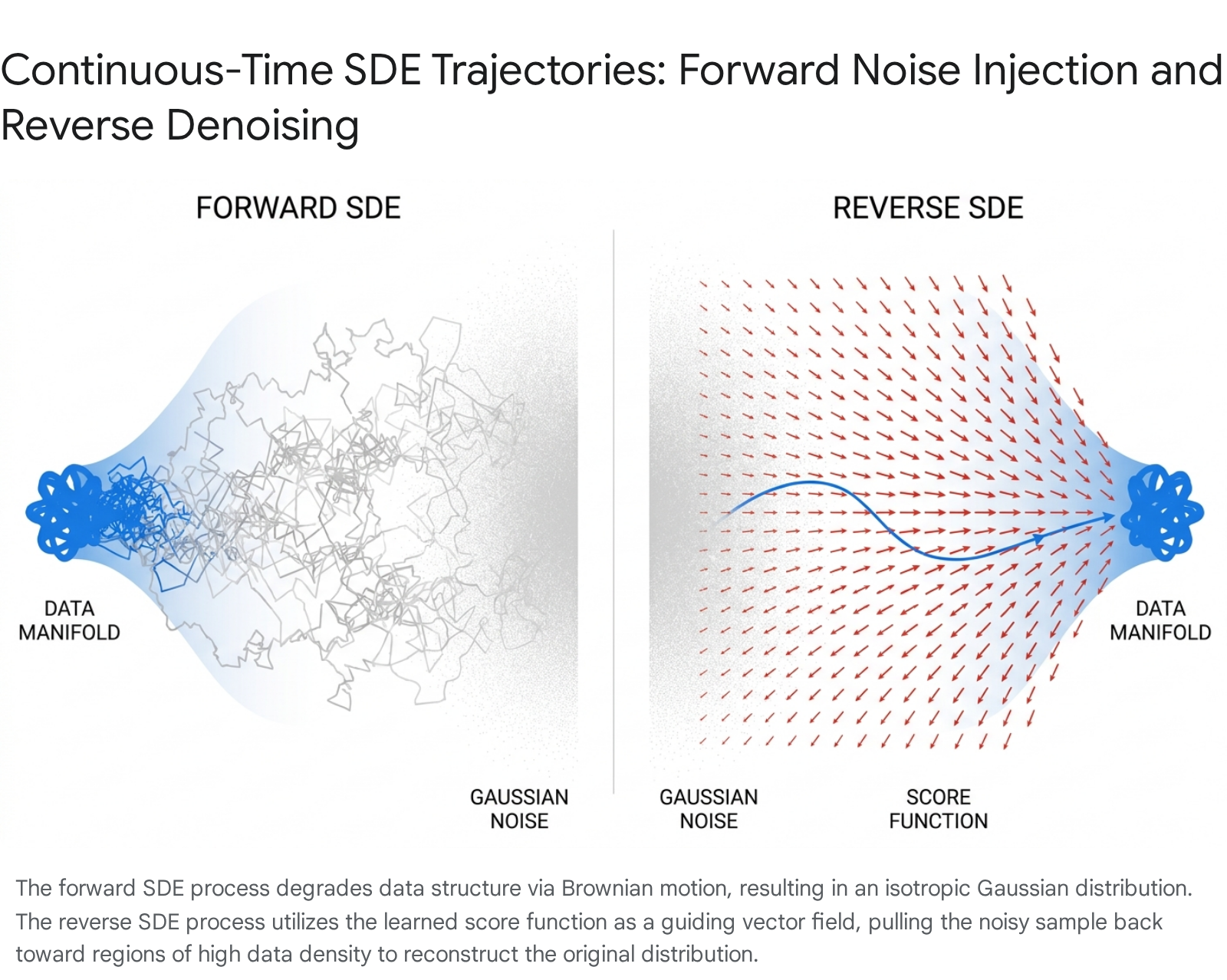
During the Forward Noising Trajectory, the process initiates from a point located on the highly concentrated, sharp data manifold - for instance, a specific configuration of pixels representing a highly detailed image of a face. The forward trajectory operates as a constrained random walk. At each infinitesimal time step, the Brownian motion component ($g(t)dw$) causes the particle to diffuse outward randomly, injecting chaotic energy into the system 410. Simultaneously, in the VP formulation, the deterministic drift term ($f(x, t)dt$) constantly pulls the particle gently toward the origin. Over continuous time, the highly localized and complex data density diffuses, systematically smoothing out high-frequency details. Eventually, the entire distribution topologically morphs into a structureless, isotropic Gaussian noise ball 410.
Conversely, during the Reverse Denoising Trajectory, the process initiates from a random coordinate within the isotropic Gaussian noise distribution. Unlike the forward process, the reverse trajectory is not a random walk; rather, it utilizes the learned score function to establish a highly structured, deterministic vector field. At every infinitesimal step backward in time, the vector field $\nabla_x \log p_t(x)$ points strictly in the direction of increasing data likelihood 89. The particle is forcefully pulled out of the uniform noise cloud, navigating complex topological contours and overcoming the inherent stochasticity of the reverse Brownian motion. Guided entirely by the neural network's gradient estimations, the trajectory smoothly maneuvers the particle to settle precisely within the sharp, distinct boundaries of the original data manifold.
Architectural Scope: From Pixel Space to Latent-Space Transformers
As the theoretical underpinnings of continuous-time diffusion models reached maturity, computational pragmatism mandated severe architectural shifts in how these models were physically constructed and deployed. The most significant of these shifts involved relocating the computationally intensive diffusion process from high-dimensional pixel space to a highly compressed latent space, followed by the replacement of traditional convolutional U-Nets with highly scalable Vision Transformer architectures.
Differentiating Pixel-Space and Latent-Space Diffusion
Standard DDPMs, as originally proposed, operate directly in pixel space. This requires the neural network to evaluate and predict noise across every single pixel, across all three RGB color channels, for hundreds of sequential timesteps 15. For high-resolution image synthesis, this pixel-level evaluation results in exorbitant computational costs, rendering both training and inference exceedingly slow and resource-intensive 315.
Latent Diffusion Models, introduced to solve this bottleneck, fundamentally bifurcate the generative process into two discrete, sequential stages: semantic compression and generative diffusion 1520. It is an exceedingly common error to conflate the Variational Autoencoder component with the diffusion process itself; however, their roles are mathematically and functionally distinct.
The first stage utilizes a pretrained VAE to handle perceptual compression 32021. The encoder transforms the high-dimensional image into a significantly lower-dimensional latent representation 321. Crucially, the VAE is responsible for filtering out imperceptible, semantically meaningless high-frequency details from the image 1516. The VAE's loss function is strictly based on spatial reconstruction error alongside KL divergence to regularize the latent manifold into a roughly normal distribution 21. Recent research emphasizes that a generation-friendly VAE must excel at semantic disentanglement, capturing attribute-level meaning rather than mere pixel-level reconstruction 16.
The second stage is the diffusion component, which serves as the generative engine. This diffusion process occurs entirely within the compressed latent space provided by the VAE 321. The diffusion model is completely blind to actual pixels; it learns exclusively to reverse the forward noising process on the compact latent tensors 3. By separating perceptual compression from semantic generation, LDMs execute the computationally heavy Markov chain in a space up to 64 times smaller than the original image, achieving near-optimal equilibrium between computational efficiency and high-fidelity detail preservation 315.
The Industry Shift: From U-Nets to Diffusion Transformers
Historically, the denoising networks within diffusion models overwhelmingly relied on U-Net architectures equipped with complex spatial convolutions and localized cross-attention mechanisms 151724. However, as the industry sought greater scalability and attempted to apply scaling laws to generative vision models, the inherent inductive biases of convolutions proved limiting. The paradigm has now forcefully shifted toward Diffusion Transformers 171826.
Introduced as a novel architectural class, DiTs entirely replace the U-Net backbone with a standard Vision Transformer architecture specifically modified to handle diffusion processes 1718. To process images, the latent tensor produced by the VAE is divided into non-overlapping patches, flattened, and projected into a sequence of tokens, directly mirroring the standard ViT natural language pipeline 1718.
A core innovation in the DiT design is its approach to conditioning. Diffusion timesteps and class labels are not embedded via traditional cross-attention layers inserted between convolutional blocks. Instead, they are injected directly into the transformer blocks using adaptive layer normalization (adaLN) 17. The network predicts the precise scale and shift parameters for the layer normalization operation directly from the sum of the timestep and conditioning embeddings 17. The most compelling argument for the adoption of DiTs is their highly predictable scaling behavior. Empirical analyses demonstrate a direct, inverse correlation between forward pass complexity (measured in Gflops) and sample quality (measured by Fréchet Inception Distance). Consequently, increasing transformer depth, width, or input token count consistently yields proportionally lower FID scores, validating the transformer architecture's supremacy for generative scaling 171819.
Multimodal DiTs and Advanced Video Generation
The baseline DiT architecture has further evolved to accommodate complex, multi-modal synthesis, most notably observed in text-to-image systems like Stable Diffusion 3 and text-to-video systems like OpenAI's Sora 2820.
Standard cross-attention mechanisms artificially force text embeddings into an image-dominant convolutional stream, often leading to poor prompt adherence. Stable Diffusion 3 addresses this fundamental mismatch with the Multimodal Diffusion Transformer (MM-DiT). Recognizing that text and image embeddings belong to conceptually disparate modalities with unique internal structures, MM-DiT employs two entirely separate sets of weights for processing image and language tokens 2420. The streams remain fully independent through the Query, Key, and Value projection phases. However, they are concatenated specifically for a unified joint-attention operation 30. This sophisticated design allows both modalities to operate in their native representational spaces while ensuring unrestricted bidirectional information flow. The result is a drastic improvement in complex text comprehension and the ability to generate accurate typography - a historical weakness of U-Net-based models 203021.
OpenAI's Sora further extends the diffusion transformer framework to tackle the immense complexity of video generation. Processing video requires managing an exponential increase in token volume over time. Sora achieves this by utilizing a deep video compression network to map raw video frames into a latent space, followed by the extraction of "spacetime latent patches" 2822. By utilizing techniques akin to Tubelet embeddings - where spatial patches and temporal frames are fused simultaneously into a single, unified token - the model inherently grasps the continuity of physical motion 28. This patch-and-pack tokenization strategy allows the DiT architecture to seamlessly process highly variable resolutions, aspect ratios, and video durations without relying on the rigid temporal convolutions that constrained prior video generation systems 28.
Computational Limitations and Mitigation Strategies
Despite their supreme generative fidelity and robust theoretical backing, standard diffusion models suffer from a debilitating computational bottleneck: the massive Number of Function Evaluations (NFE) required during the reverse sampling phase 233435. Because the reverse SDE or ODE must be solved numerically over hundreds or even thousands of discrete timesteps (e.g., $T=1000$ to $2000$), generating a single image is orders of magnitude slower than the single forward pass of a GAN or VAE 363738. Addressing this latency has been the primary focus of recent generative research.
Denoising Diffusion Implicit Models (DDIM)
The introduction of Denoising Diffusion Implicit Models fundamentally altered the landscape of diffusion sampling by proving that the forward process does not actually need to be Markovian to yield the exact same marginal distributions as DDPMs 3940. DDIM generalizes the reverse step computation by introducing a variance parameter, denoted as $\eta$, which dictates the stochasticity of the trajectory 39.
When $\eta=1$, the generative process remains strictly stochastic, adding random Gaussian noise at every step and mathematically mirroring the standard DDPM 3941. However, when $\eta=0$, the noise injection term vanishes entirely, converting the reverse trajectory from a random walk into a completely deterministic Probability Flow Ordinary Differential Equation 3942.
This determinism allows DDIM to drastically decouple the generation step size from the highly granular training schedule. Instead of stubbornly evaluating all 1,000 steps, DDIM allows the model to traverse a subsequence of the timesteps, taking significantly larger analytical strides through the latent space 3940. As a result, DDIM can synthesize high-fidelity samples in as few as 50 to 100 steps, effectively accelerating inference by a factor of ten to twenty without requiring any retraining of the base neural network 3940. Furthermore, because the generative path is completely deterministic for a given initial noise vector, DDIM uniquely enables exact latent space interpolation, semantic editing, and consistent inversion techniques that are impossible under stochastic DDPMs 3941.
Flow Matching and Rectified Flow
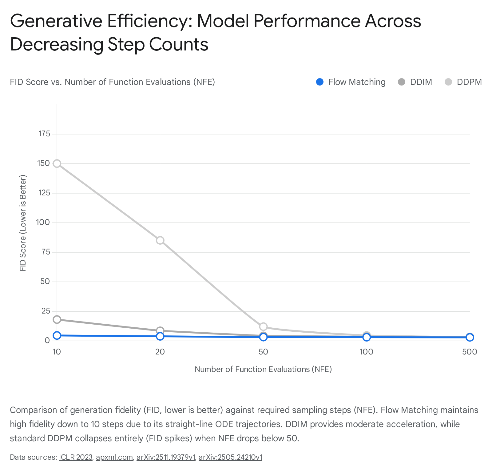
While DDIM successfully accelerates sampling, the underlying probability paths dictated by standard Variance Preserving and Variance Exploding SDEs remain mathematically suboptimal. Analysis of these paths reveals that they are inherently highly curved and tortuous, often exhibiting a geometric curvature metric ($\mathcal{C}$) of approximately 3.45 34. Because curved paths inherently incur severe discretization errors when simulated with large step sizes, there is a hard limit to the maximum achievable speed-up; pushing step counts too low causes the numerical solver to veer off the manifold entirely, resulting in image collapse 3424.
Rectified Flow, and the broader theoretical umbrella of Flow Matching, provides an elegant mathematical solution to this geometric problem. Instead of relying on predefined diffusion physics, Flow Matching actively forces the generative ODE to follow the shortest possible straight-line paths connecting the prior noise distribution ($\pi_0$) directly to the target data distribution ($\pi_1$) 2425454647.
The Rectified Flow training objective is achieved through a straightforward nonlinear least squares optimization problem that minimizes the difference between the network's predicted velocity field and the ideal linear trajectory equation: $X_t = t X_1 + (1-t)X_0$ 2446. Because the model is explicitly trained to learn a highly laminar vector field with near-zero second derivatives ($d^2x/dt^2 \approx 0$), the geometric curvature of the sampling path is almost entirely neutralized, resulting in a remarkably low curvature metric of $\mathcal{C} \approx 1.02$ 34.
This extreme path rectification yields profound computational benefits. It allows exceptionally simple, lightweight first-order numerical solvers, such as the Euler method, to traverse the generation trajectory with massive step sizes without accumulating the severe integration errors that plague curved diffusion paths 3424. Flow Matching establishes a new "efficiency frontier" in generative AI, capable of producing coherent, sharp, high-fidelity samples in as few as $N=10$ function evaluations 3435. This is a critical threshold where standard DDPM and DDIM formulations collapse completely into unstructured noise, cementing Flow Matching as the definitive framework for the next generation of efficient models, including architectures like Stable Diffusion 3 243435.
Comparative Analysis of Generative Frameworks
To fully contextualize the current state of generative AI, one must objectively compare the mathematical, structural, and performance trade-offs governing architecture choice and sampling techniques across the broader machine learning landscape.
The Generative Learning Trilemma: Diffusion vs. GANs vs. VAEs
The foundational models in generative learning face an inherent set of compromises often referred to as the generative learning trilemma. This principle proposes that models typically struggle to simultaneously achieve high sampling speed, high generative fidelity, and robust diversity or mode coverage 2649. Table 1 concisely illustrates how different foundational paradigms navigate these engineering compromises based on topological constraints and training methodologies.
Table 1: Generative Paradigms: Diffusion Models vs. GANs vs. VAEs
| Feature | Diffusion Models | Generative Adversarial Networks (GANs) | Variational Autoencoders (VAEs) |
|---|---|---|---|
| Mathematical Basis | Iterative denoising via Markov chains / SDEs | Adversarial min-max game (Generator vs. Discriminator) | Probabilistic latent manifold regularization via ELBO |
| Output Fidelity | Extremely High (State-of-the-art detail and texture) | Extremely High (Photorealistic, extremely sharp) | Moderate to Low (Prone to blurry, averaged outputs) |
| Diversity (Mode Coverage) | Excellent (Robustly covers the entire data distribution) | Poor (Highly prone to severe mode collapse) | Excellent (Produces smooth, continuous interpolations) |
| Training Stability | Highly Stable (Relies on simple MSE regression objectives) | Highly Unstable (Requires careful hyperparameter balancing) | Highly Stable (Clear probabilistic convergence) |
| Inference Speed | Very Slow (Requires multiple sequential NFE passes) | Very Fast (Single forward pass network execution) | Very Fast (Single forward pass network execution) |
| Primary Use Cases | High-fidelity text-to-image/video, complex spatial generation | Real-time generation, interactive synthesis, deepfakes | Representation learning, anomaly detection, data compression |
Generative Adversarial Networks excel immensely in computational speed and visual sharpness because they generate complete data samples in a single forward pass through a generator network 365051. However, GANs fundamentally lack an explicit likelihood model and rely on an inherently unstable adversarial zero-sum game 5052. This leaves them exceptionally vulnerable to mode collapse - a catastrophic failure wherein the generator discovers a tiny subset of the data distribution that successfully tricks the discriminator and subsequently memorizes it, failing to represent the true diversity of the training data 38505152. Furthermore, ensuring stable convergence in GANs requires complex gradient penalties and spectral normalizations that often feel more like art than rigorous science 5051.
Conversely, Variational Autoencoders solve the stability and diversity problems by imposing a strict probabilistic structure on the latent space 21384953. They ensure robust coverage and smooth interpolations but suffer from consistently blurry outputs because their reconstruction loss mathematically averages over overlapping modes in the data distribution 21384953. Diffusion models emerged as the dominant framework by solving the fidelity and diversity constraints concurrently 264952. By learning to slowly reverse a systematic degradation process via simple regression targets, diffusion models achieve the visual sharpness of GANs while maintaining the comprehensive mode coverage and training stability of VAEs, albeit by sacrificing inference velocity 264952.
Optimization in Sampling: DDPM vs. DDIM vs. Flow Matching
While Diffusion remains the dominant overall paradigm for image and video synthesis, the mathematical mechanics driving the reverse synthesis phase have heavily fractured into distinct methodologies, each aggressively optimized for latency reduction and edge-device deployment. Table 2 contrasts the primary sampling frameworks utilized to solve the continuous or discrete generative trajectories.
Table 2: Evolution of Diffusion Sampling Frameworks
| Metric / Feature | Standard DDPM | DDIM ($\eta = 0$) | Flow Matching / Rectified Flow |
|---|---|---|---|
| Mathematical Pathway | Stochastic Differential Equation (SDE) | Probability Flow ODE | Transport Mapping ODE |
| Determinism | Inherently Stochastic (Adds variance at every step) | Fully Deterministic (Noise scaling set to zero) | Fully Deterministic (Straight-line vector field) |
| Path Curvature ($\mathcal{C}$) | Highly tortuous ($\mathcal{C} \approx 3.45$) | Moderate to High curvature | Near-linear / Straighter paths ($\mathcal{C} \approx 1.02$) |
| Sampling Steps (NFE) | 250 - 1000+ (Requires dense integration) | 50 - 200 (Allows sub-sequence jumps) | 1 - 20 (Allows massive integration steps) |
| Truncation Resilience | Fails entirely below $N=50$ (Outputs pure noise) | Degrades visually below $N=20$ (Artifact introduction) | Maintains recognizable fidelity at $N=10$ |
| Solver Dependency | Langevin-style ancestral sampling | Flexible step-size ODE solvers | Lightweight 1st-order Euler solvers |
The progression from standard DDPM to DDIM and ultimately to Flow Matching illustrates a highly deliberate engineering trajectory aimed at eliminating the computational bottlenecks of generative AI. By eliminating stochasticity with DDIM and actively penalizing geometric curvature during the training phase with Rectified Flow, researchers have successfully bridged the gap between the unparalleled quality of iterative diffusion modeling and the real-time inference speeds traditionally monopolized by single-pass networks 344124. Flow Matching, in particular, represents a pinnacle in this progression, ensuring that generation trajectories are not merely effective, but mathematically optimal in their routing through the latent space 18342447.
Conclusion
The current state of deep generative modeling is defined by an unprecedented synthesis of rigorous, physics-based probability theory and massive-scale engineering. The mathematical unification of standard Denoising Diffusion Probabilistic Models and Score-Based Generative Models under the Continuous-Time Stochastic Differential Equation framework provided the exact theoretical bedrock necessary to explore arbitrary forward dynamics and optimal reverse trajectories via Tweedie's formula. Meanwhile, acute computational pragmatism drove a massive architectural shift away from pixel-space U-Nets toward Latent-Space Multimodal Diffusion Transformers, permanently divorcing semantic perceptual compression from the generative diffusion engine to unlock massive scalability.
As the industry aggressively targets real-time video generation and edge-device deployment, the geometric optimization of the reverse sampling trajectory has become the primary vector of theoretical innovation. By replacing highly curved, stochastically inefficient random walks with the deterministic, straight-line ODE trajectories of Flow Matching, modern architectures possess the capability to yield state-of-the-art fidelity at a sheer fraction of historical computational costs. This convergence of optimized inference latency, predictable transformer-driven scaling laws, and continuous-time mathematics dictates that the generative models of the immediate future will not only be exponentially more expressive but structurally bound to unprecedented levels of computational efficiency.