Loss Landscape Geometry in Neural Networks
Introduction to High-Dimensional Loss Topologies
In the domain of machine learning, the process of training a neural network is fundamentally a mathematical optimization problem defined over a highly complex, non-convex parameter space. The loss landscape is the high-dimensional surface mapping a model's parameters - its specific configurations of weights and biases - to a scalar loss value. This loss value represents the quantitative discrepancy between the model's predictions and the true target values within a dataset 12. For a deep neural network consisting of $N$ parameters, this landscape exists as a geometric object within an $(N+1)$-dimensional space 32. The central objective of optimization algorithms, such as Stochastic Gradient Descent (SGD) and its adaptive variants, is to navigate this extraordinarily high-dimensional terrain to identify coordinate vectors that globally, or at least optimally locally, minimize the objective function 236.
Historically, the scientific intuition governing optimization theory was heavily drawn from low-dimensional, strictly convex problems. In these classical settings, the loss surface resembles a simple two- or three-dimensional parabolic bowl where gravity-like gradient flow inevitably terminates at a single, easily identifiable global minimum 23. However, modern deep learning architectures - ranging from wide convolutional networks to massive attention-based Transformers - frequently possess parameter counts extending into the billions 13. This explosion in scale forces the objective function into an extreme high-dimensional regime where classical intuitions break down entirely 7. In this regime, the geometry of the space dictates every critical aspect of neural network training: whether a model's gradients will vanish or explode, the speed at which the optimizer converges, and, most crucially, how effectively the resulting parameter configuration will generalize to unseen data distributions 45.
The contemporary understanding of loss landscape geometry has shifted decisively away from the early fear of ubiquitous, poor local minima. Instead, researchers conceptualize the space through a framework characterized by an overwhelming abundance of saddle points, multiscale valley structures, highly degenerate parameter regions, and interconnected manifolds of low loss 467. Furthermore, recent theoretical advancements - particularly those rooted in singular learning theory, optimal transport, and topological data analysis - have begun linking the specific geometric curvature of these landscapes to complex, emergent behavioral phenomena. These include stagewise heuristic development, the double descent generalization curve, and the delayed generalization phenomenon known as grokking 1289. Understanding the topography of these landscapes is therefore not merely an exercise in numerical analysis, but the foundational key to unlocking why deep learning functions effectively in practice.
Mathematical Caveats and the Curse of Dimensionality
Analyzing the geometry of neural networks presents severe visualization and analytical challenges. Because human spatial intuition is strictly confined to three physical dimensions, researchers are forced to utilize extreme low-dimensional projections to probe the landscape. Typically, these visualizations take the form of one-dimensional linear interpolations between two parameter vectors, or two-dimensional cross-sections defined by random or gradient-aligned direction vectors 151011. While these projections yield valuable insights, they are accompanied by profound mathematical caveats dictated by the nature of high-dimensional geometry.
The Curse of Dimensionality and Empty Space Phenomena
The "curse of dimensionality," a term originally coined by mathematician Richard E. Bellman in 1957, refers to the counterintuitive phenomena that arise when analyzing data in spaces with hundreds, thousands, or millions of dimensions 121813. The primary driver of this curse in the context of loss landscapes is the exponential scaling of volume, which leads to the "empty space phenomenon" 1314.
In low dimensions, a dataset can adequately cover the parameter space. However, as dimensions scale, the volume of the space grows so rapidly that the parameter space becomes statistically sparse 1218. To illustrate the geometric betrayal of high dimensions, consider a unit hypercube (sides of length 1) and a slightly smaller hypercube inside it (sides of length 0.9). In one dimension, the smaller segment occupies 90% of the volume. In two dimensions, it occupies 81% ($0.9^2$). In three dimensions, it occupies 72.9% ($0.9^3$). By the time the space reaches merely 100 dimensions - a minuscule number compared to modern neural networks - the smaller hypercube occupies approximately $0.0026\%$ ($0.9^{100}$) of the original volume 13. Consequently, in the millions of dimensions of a neural network loss landscape, almost all the volume of the space is concentrated in the extreme corners of the hypercube rather than the center 14.
Furthermore, the concept of Euclidean distance severely distorts as dimensions scale. The phenomenon of "distance concentration" guarantees that the Euclidean distance between almost any two randomly selected points approaches a similar, extremely high constant value 1315. Mathematically, as dimensionality approaches infinity, the ratio of the distance to the nearest point to the distance to the farthest point converges exactly to 1 1315. Random vectors generated in high-dimensional spaces are also almost always perfectly orthogonal to one another 14. Because of these geometric realities, taking a random 2D slice of a 10-million-dimensional space captures a microscopically specific, flat planar trajectory that is fundamentally blind to the vast, complex ridges and valleys situated in the orthogonal 9,999,998 dimensions 125.
Dimensional Projections, Scale Invariance, and Filter Normalization
To generate 3D topographical maps of the loss surface, researchers commonly select a central point in the parameter space - such as the final trained weights - and generate two random, orthogonal high-dimensional direction vectors 1022. The model's loss is then iteratively evaluated across the 2D grid plane defined by these vectors 1022. However, this standard projection methodology frequently generates mathematical mirages due to the property of scale invariance inherent in modern neural network architectures 1011.
Deep neural networks utilizing standard non-linear activation functions (such as ReLUs) exhibit positive scale invariance. If the weights in one layer are multiplied by a scalar $\alpha$, and the weights in the subsequent layer are divided by the exact same scalar $\alpha$, the functional output of the network, and thereby its loss, remains perfectly unchanged 610. While the network's predictive function is identical, the geometric representation of the weights has shifted drastically. A network with artificially scaled-up weights will compress the relative mathematical impact of the random directional perturbation 10. Consequently, without normalization, the loss landscape for the scaled model will appear artificially flat and smooth, suggesting a wide minimum, while a model with smaller weights will appear to sit in a sharp, chaotic ravine, even though both models are functionally identical 1011.
To resolve this geometric distortion, Li et al. (2018) introduced "Filter Normalization." This critical methodology ensures that the randomly generated perturbation directions are normalized to match the exact mathematical scale (the norm) of the specific filters or neurons they are perturbing 21011. By ensuring that perturbations are strictly proportional to the learned parameter magnitudes, filter-wise normalization guarantees that visual comparisons between different architectural configurations - or models trained under different regularization regimes - reflect genuine topological differences rather than artifacts of weight scaling 21011.
Projection Ambiguity and Trajectory Tracking
A secondary mathematical caveat of dimensionality reduction involves the mapping of optimization trajectories onto these visual planes. Because the projection from a high-dimensional parameter space down to a 2D visualization plane is a many-to-one mapping, multiple distinct high-dimensional coordinate vectors inevitably project onto the exact same low-dimensional point 16.
When researchers plot the historical trajectory of an optimizer (like SGD) onto the final filter-normalized loss landscape, they often observe a discrepancy. Despite having identical coordinates in the low-dimensional projection space, the projected points correspond to entirely distinct loss values in the true high-dimensional space 16. The optimizer may appear to be moving across a flat plateau or traversing uphill in the 2D projection, even when the true high-dimensional trajectory was strictly following a steep gradient descent 16. Therefore, visual landscapes inherently view the "current" central point as a local minimum, masking the true direction of optimization reduction that was accessible during earlier stages of training 16.
Topological Features: Minima, Saddle Points, and Multiscale Structures
The topology of the neural network loss landscape is uniquely perilous for standard optimization algorithms. Understanding how optimizers successfully navigate this terrain requires redefining the types of critical points that dominate the parameter space.
The Extreme Prevalence of Saddle Points
Early deep learning theory operated under the assumption that the primary barrier to training was the existence of numerous poor local minima - suboptimal basins where the algorithm would become irreversibly trapped 34. However, random matrix theory and advanced geometric analyses have conclusively demonstrated that in the highly over-parameterized settings of deep neural networks, true local minima are mathematically scarce. Instead, the landscape is overwhelmingly dominated by saddle points 3417.
A critical point occurs wherever the first-order gradient of the loss function vanishes ($\nabla L(\theta) = 0$). For this critical point to be classified as a local minimum, the Hessian matrix - the $N \times N$ square matrix of second-order partial derivatives representing the local curvature of the space - must be strictly positive semi-definite 34. This requires every single eigenvalue of the Hessian to be greater than or equal to zero 3417.
As the dimensionality of the model scales into the millions, the statistical probability that every independent eigenvalue of the Hessian happens to be randomly positive decreases exponentially toward zero 417. Consequently, almost all critical points encountered in high-dimensional optimization are saddle points. At a saddle point, the Hessian exhibits a mixture of positive and negative eigenvalues. The surface curves upward in certain parameter dimensions (resembling a minimum) and curves downward in orthogonal dimensions (resembling a maximum), creating a geometry akin to a mountain pass or a horse's saddle 31718.
Algorithmic Escapes from Degenerate Regions
The prevalence of saddle points poses a severe mechanical threat to first-order optimization algorithms like standard Gradient Descent (GD). Because the gradient approaches zero near a saddle point, the algorithm's step size shrinks infinitesimally, causing progress to stall drastically 317. This stall creates the illusion of convergence; the loss plateaus for dozens of epochs, and the model appears to have finished training when it is actually merely wandering aimlessly across a highly degenerate, flat region of mixed curvature 1718.
Escaping these regions necessitates specific optimization dynamics. The stochasticity inherent in mini-batch Stochastic Gradient Descent (SGD) is critical. By calculating gradients on random subsets of data rather than the full population, SGD injects continual mathematical noise into the optimization trajectory 171819. This random perturbation prevents the optimizer from settling precisely on the zero-gradient saddle, eventually pushing the parameters into a dimension of negative curvature, allowing the loss to drop rapidly 1827.
Furthermore, adaptive optimizers such as Adam and RMSProp explicitly counter saddle geometry by scaling updates on a per-parameter basis 11719. By dividing the learning rate by the moving average of the squared gradients, these optimizers amplify the step size in flat directions (where gradients are small) and dampen the step size in steep directions. This accelerates the algorithm's escape from saddle regions, a mechanism that contributes heavily to the ubiquity of Adam in modern deep learning 11719.
Multiscale Structures and the Edge of Stability
Beyond the localized geometry of saddle points, the loss landscape exhibits a complex "multiscale" structural hierarchy. Extensive research reveals that beyond the immediate microscopic neighborhood of a minimum, the loss landscape violates standard quadratic approximations (Taylor expansions) entirely 6. Instead, it exhibits subquadratic growth characterized by separate, distinct scales: narrow, sharp wells are frequently nested deeply within much broader, flatter macro-valleys 6.
This multiscale topography heavily influences the dynamics of the learning rate. When gradient descent operates with a relatively large learning rate ($\eta$), it possesses too much kinetic energy to settle into the sharp, narrow microscopic wells. Instead, the optimizer oscillates violently from wall to wall within the sharp features - a phenomenon rigorously defined as operating on the "Edge of Stability" 6. In a purely quadratic landscape, this instability would cause the loss to explode to infinity. However, because neural network landscapes are subquadratic, the optimizer stabilizes, bouncing along the walls while migrating slowly down the broader, large-scale manifold of the macro-valley 6.
This dynamic implies that the loss landscape fundamentally dictates the timing of Learning Rate Decay (LRD) schedules. If the learning rate is decayed prematurely, the optimizer loses its energy and plunges into the nearest sharp, suboptimal well, becoming trapped. If the learning rate remains high, the optimizer systematically avoids the sharpest regions (where the localized curvature exceeds $2/\eta$) and favors broader, more robust regions of the space 6.
| Topological Feature | Geometric Description | Optimization Challenge | Algorithmic Mitigation |
|---|---|---|---|
| Saddle Point | Critical point with zero gradient and mixed Hessian curvature (eigenvalues of mixed signs). | Causes first-order optimizers to stall entirely, creating false plateaus in the loss curve. | SGD mini-batch noise; Momentum accumulation; Adaptive learning rates (Adam). |
| Sharp Minimum | Deep, narrow convergence well characterized by large Hessian eigenvalues. | Highly sensitive to small parameter perturbations; associated with poor generalization. | Large learning rates (Edge of Stability); Sharpness-Aware Minimization (SAM). |
| Flat Minimum | Broad basin with near-zero curvature across many parameter dimensions. | Difficult to locate quickly due to vanishing gradients in the flat basin. | Trust-region methods; Cyclical learning rate schedules. |
| Poor Local Minimum | Suboptimal basin where all curvature directions are strictly positive. | Prevents the algorithm from reaching the global minimum. | Avoided naturally in high-D via massive over-parameterization. |
The Flatness Hypothesis and Generalization
A central, unresolved mystery in deep learning theory is why highly over-parameterized models - which possess enough mathematical capacity to perfectly memorize random noise - consistently manage to generalize to unseen test data. The most prominent geometric explanation bridging optimization and generalization is the Flat Minima Hypothesis.
The Mechanics of Sharp vs. Flat Minima
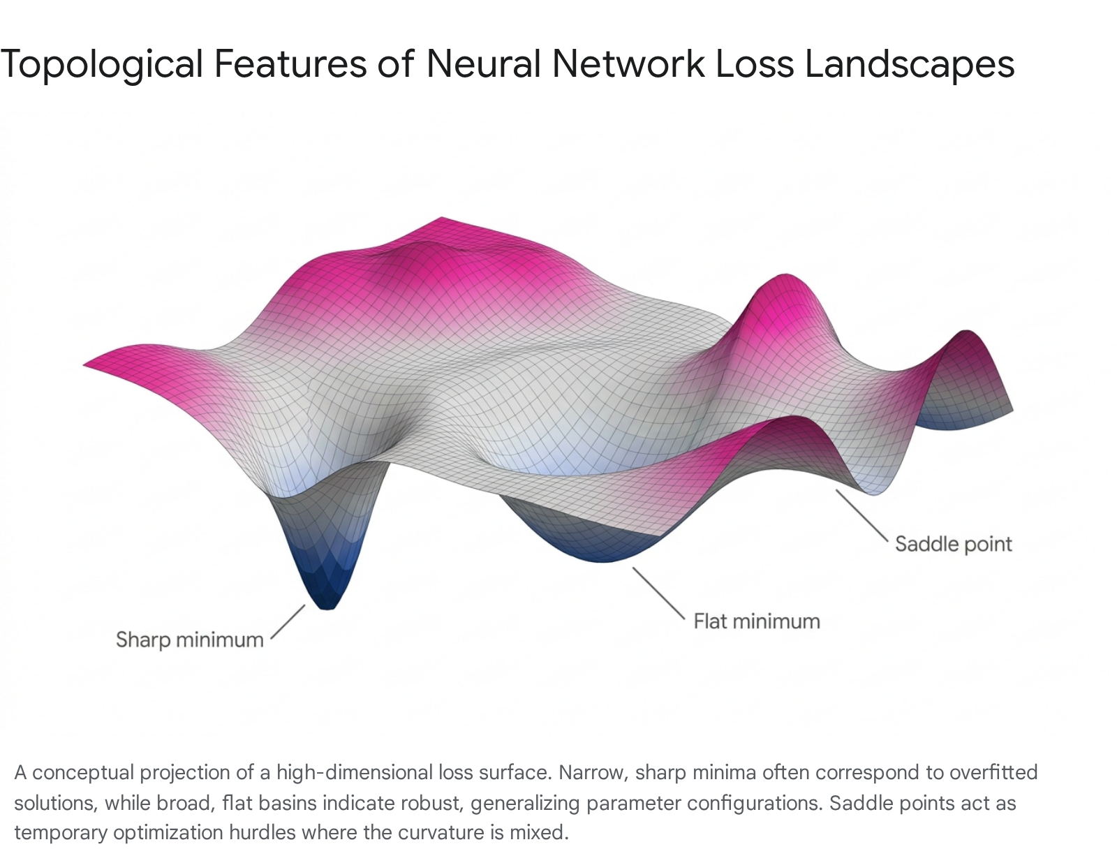
The local topology of the final convergence point heavily dictates a model's robustness and out-of-distribution performance. A "sharp" minimum corresponds to a region of parameter space with exceptionally high curvature, characterized by a large top eigenvalue of the Hessian matrix 11720. In a sharp minimum, the loss function resembles a steep ravine; a microscopic perturbation in the model's weights results in a massive spike in the loss value 1720. Conversely, a "flat" minimum is a broad, shallow basin where the curvature is near zero across the majority of spatial dimensions. Here, the weights can be altered significantly without materially affecting the network's predictive loss 1720.
Flat minima are heavily correlated with superior generalization. This can be understood through the lens of the Minimum Description Length (MDL) theory. Parameters residing in a flat minimum require significantly less numerical precision to specify (e.g., a weight of 0.1 performs identically to a weight of 0.1001), indicating lower absolute model complexity and a reduced propensity to overfit to the exact noise characteristics of the training data 20. Furthermore, flat minima provide natural robustness to distributional shifts between the empirical training data and the actual test data. A shift in data distribution effectively translates the physical location of the loss landscape. If a model rests in a broad, flat basin, a slight shift in the landscape ensures the parameters still evaluate to a low loss. If the model rests in a sharp, narrow ravine, that same geometric shift will pull the ravine entirely out from under the parameters, resulting in a catastrophic loss spike on the test set 1820.
Empirical findings strongly support this correlation. Training regimens utilizing exceptionally large batch sizes calculate highly accurate gradients that swiftly pull the optimizer into the nearest sharp minimum, resulting in models that fail to generalize 182021. Conversely, small batch sizes induce significant stochastic noise, actively preventing the optimizer from settling in sharp ravines and effectively forcing it to wander until it locates a broad, noise-tolerant flat minimum 182021.
Sharpness-Aware Minimization (SAM) and its Critiques
To explicitly engineer this geometric outcome, optimization algorithms like Sharpness-Aware Minimization (SAM) and Sharpness-Aware Gradient Descent (SA-GD) were developed. Rather than simply seeking to minimize the current loss, SAM operates by seeking parameter values whose entire spatial neighborhood possesses uniformly low loss 12030. Mathematically, SAM achieves this by taking an adversarial ascent step to find the point of maximal loss within a predefined neighborhood radius $\rho$, and then calculating the gradient descent step from that adversarial point 203031.
Despite the empirical success of SAM across diverse architectures, recent rigorous analytical studies have surfaced significant critiques regarding the absolute theoretical link between flatness and generalization. Studies evaluating the canonical setting of stochastic convex optimization have demonstrated that the relationship is subtly dependent on the precise data distribution and model architecture 303122.
The critiques reveal a fracture in the flatness hypothesis. Researchers have mathematically proven that flat empirical minima can sometimes incur a trivial, poor population risk (denoted as $\Omega(1)$ risk), while sharp minima can, in certain specific configurations, generalize optimally 3031. Furthermore, algorithms explicitly designed to hunt for flatness possess their own algorithmic blind spots. SAM, despite serving as a computationally efficient approximation of SA-GD, can sometimes successfully minimize empirical loss while failing entirely to avoid sharp minima 3031. Similarly, SA-GD can provably converge at a fast rate to flat minima that generalize strictly worse than solutions found by standard, non-sharpness-aware SGD 3031.
Interestingly, deep investigations into the training dynamics of SAM reveal an implicit geometric bias occurring strictly late in training. Applying SAM for merely a few epochs at the very end of a standard SGD training run yields nearly identical generalization benefits and solution sharpness to utilizing full SAM training from initialization 23. This highlights a two-phase dynamic where late-phase SAM exponentially rapidly escapes the sharp minimum discovered by SGD, and shifts rapidly to a flatter minimum localized within the exact same macro-valley 23. This implies that early-stage optimization is necessary to locate the correct general basin, while sharpness penalization is only required to adjust the final resting coordinates within that basin.
The Geometry of Double Descent
The relationship between landscape geometry, model capacity, and generalization is most strikingly visible in the "double descent" phenomenon 3424. Classical statistical learning theory dictates a strict U-shaped bias-variance tradeoff: as model complexity increases, training error drops, but test error eventually spikes as the model begins overfitting to training noise 3424. The classical recommendation is to halt capacity expansion at the bottom of the U-curve.
In modern, over-parameterized neural networks, increasing capacity yields a radically different trajectory. The first phase follows classical theory: in the under-parameterized regime, as parameters increase, test and training error both decrease. However, as the network reaches the "interpolation threshold" - the exact critical capacity point at which the model has just enough parameters to perfectly memorize the entire training dataset - the test error predictably spikes to a massive peak, seemingly validating the classical overfitting hypothesis 3424.
Yet, as capacity is aggressively increased past this threshold, adding parameters well beyond the number of data points, the test error unexpectedly descends a second time, frequently achieving performance far superior to the optimal point of the classical under-parameterized regime 3424.
The driving mechanism behind double descent is entirely geometric. By visualizing the filter-normalized loss surface across the double descent curve, researchers demonstrate that the geometry of the minimizer changes radically. At the exact interpolation threshold, the model is forced to utilize every available parameter to fit the data, resulting in a highly constrained solution. In the loss landscape, this corresponds to the absolute sharpest, narrowest minimum across the entire capacity spectrum 34.
As the model pushes deeper into the over-parameterized regime, the excess parameters are no longer strictly required to fit the data. Instead, they manifest mathematically as vast, degenerate directions of zero curvature within the Hessian matrix. The sharp ravines physically stretch out, and the basins of convergence become massively widened and flattened 3424. The double descent phenomenon proves that extreme complexity, counter to classical intuition, generates a highly degenerate, perfectly flat loss landscape that implicitly regularizes the model and inherently protects against overfitting 3424.
Manifolds, Symmetries, and Linear Mode Connectivity
A foundational realization in high-dimensional landscape geometry is that global minima are almost never isolated points in space; rather, they form extensive, continuous manifolds spanning millions of dimensions 467.
If a neural network is trained twice using standard SGD - starting from two entirely different random initializations or utilizing different data shuffling orders - the optimizer will converge to two entirely disparate coordinate vectors in the parameter space, $\theta_A$ and $\theta_B$ 25. Traditionally, if one linearly interpolates a straight path between these two points in the parameter space, the loss value spikes massively in the middle of the path. This spike suggests that the two minima exist in completely separate, distinct geometric basins divided by an impassable high-loss barrier 726.
Permutation Invariance and Optimal Transport
However, deep neural networks possess extensive functional symmetries that complicate this spatial interpretation. Specifically, networks exhibit permutation invariance. Swapping the exact spatial positions of two neurons within a hidden layer - along with rerouting their respective incoming and outgoing weight connections - results in a numerically distinct parameter vector that produces the exact same functional output and identical loss 2527.
Recent literature has heavily investigated the phenomenon of Linear Mode Connectivity (LMC) modulo permutation. Researchers discovered that if the hidden neurons of Network B are systematically permuted to functionally align with the specific neuron roles of Network A, the perceived high-loss barrier between the two networks completely collapses 2527. Achieving this alignment is an extremely complex combinatorial problem, frequently solved by leveraging Optimal Transport theory. By applying Wasserstein distance metrics to measure and align the empirical distributions of neuron activations, researchers can compute a "soft alignment" that optimally matches the features of the distinct models 25.
Once aligned, the linear interpolation path between the two models maintains a near-zero loss barrier 2527. The two disparate solutions are thereby revealed not as isolated basins, but as points residing on the exact same vast, interconnected low-loss manifold 725. Theoretical frameworks, relying on the convergence rates of empirical measures, have rigorously proven that with high probability, any two sufficiently wide two-layer neural networks trained independently with SGD are linearly mode connected once permutation symmetries are resolved 252739. The width of the network serves as a critical geometric requirement; wider networks systematically display smaller error barriers, while extreme depth actively degrades connectivity 2527.
Layer-Wise Loss Barriers
The spatial behavior of these connections becomes highly heterogeneous when analyzed layer by layer. When models are combined for applications like federated learning, researchers explore Layer-Wise Linear Mode Connectivity (LLMC) 2628. By interpolating individual layers between two aligned networks while holding the remaining layers constant, studies demonstrate that deep networks do not distribute loss barriers evenly across their architecture.
Specifically, early layers (those adjacent to the input data) and late layers (those adjacent to the final classifier output) typically exhibit complete linear connectivity, yielding zero-loss barriers when interpolated independently 2628. Conversely, interpolating the middle layers of the exact same network consistently generates catastrophic high-loss barriers 2829. This indicates that the middle layers of a deep network act as highly sensitive representation bottlenecks. The geometric topology at these middle depths is strictly non-convex and non-linear, whereas the outer layers operate in a subspace that is effectively flat and convex 28. Furthermore, single-layer subspaces demonstrate vastly different tolerances to random noise, proving that treating random directions as uniformly representative of the global loss landscape is mathematically flawed 2829.
Loss Landscape Geometry in Transformers
The architectural dominance of the Transformer - a model relying heavily on attention mechanisms rather than recurrence or convolution - has driven intense research into how the loss landscape shapes sequence modeling, reasoning, and language acquisition. Advanced geometrical analyses demonstrate that Transformer learning dynamics are not continuous and uniform, but are instead characterized by sudden phase transitions, prolonged topological entrapments, and distinct developmental stages.
Grokking and the Commutator Defect
One of the most profound geometric anomalies observed exclusively in the loss landscapes of Transformers and certain algorithmic models is "grokking." Grokking represents the abrupt, delayed transition from rote memorization to robust generalization 830.
When a Transformer is trained on complex reasoning tasks - such as modular arithmetic, compositional language parsing (SCAN), or depth prediction (Dyck-1) - it rapidly navigates to a sharp region of the loss landscape where it effectively memorizes the training data, achieving nearly 100% training accuracy 831. At this exact point, its validation accuracy on out-of-distribution or compositional data remains at random chance 31. Over thousands, or even tens of thousands, of subsequent optimization steps, the training loss appears to plateau. However, the model is secretly traversing a highly degenerate, flat loss manifold, escaping the sharp memorization basin to physically locate a broader, generalizing circuit 83031. Suddenly, validation accuracy spikes to 100% 831.
Recent research establishes that this geometric escape is reliably preceded by specific, measurable alterations in the localized curvature of the loss landscape, quantified via the "commutator defect" 830. The commutator defect measures the non-commutativity of successive gradient updates - essentially tracking how aggressively the direction of the optimizer's movement shifts across sequential parameter updates, serving as a direct proxy for local curvature 8. Across structurally distinct task families, the commutator defect rises consistently and significantly well before the onset of generalization, providing a robust, architecture-agnostic early-warning signal that the Transformer is preparing to grok 830.
The lead time between the defect spike and actual generalization follows a strict superlinear power-law relationship (e.g., exponents of $\alpha \approx 1.18$ for SCAN and $\alpha \approx 1.13$ for Dyck datasets) 8. To prove the mechanistic validity of this topological feature, researchers conducted causal interventions in the weight space. By artificially amplifying the non-commutativity (injecting gradient noise to boost localized curvature traversal), they successfully accelerated grokking by 32% to 50%, forcing the model to escape the memorization basin faster 830. Conversely, strictly suppressing orthogonal gradient flow indefinitely trapped the Transformer in the sharp memorization basin, entirely preventing the transition to generalization 830.
Singular Learning Theory and Stagewise Development
The specific trajectory of a Transformer across the loss landscape can also be segmented using the formal framework of Singular Learning Theory (SLT). SLT posits that Bayesian inference within a neural network mathematically equates to minimizing the "free energy" over regions of parameter space, a process heavily dictated by geometric degeneracy 12. In highly degenerate spaces, large coordinate shifts in the weights yield zero change in the predictive loss.
Researchers quantify this degeneracy using the Local Learning Coefficient (LLC), a principled geometric measure of model complexity 12932. By continuously estimating the LLC and tracking its critical points over the course of training, researchers can automatically divide the optimization trajectory of an attention-only Transformer language model into discrete, rigorous developmental stages 12932.
These distinct stages, separated by critical plateaus in the loss landscape geometry, correspond perfectly to observable shifts in the model's internal computational structure. The shifting topology guides the network to sequentially learn distinct heuristics: the landscape first forces the adoption of bigram modeling, followed closely by complex n-gram generation, the activation of previous-token attention heads, and finally the formation of advanced induction heads, all before final convergence 1232. This proves that the loss landscape is not a static gradient slope, but a dynamic, evolutionary pressure that physically mandates the stagewise acquisition of linguistic capabilities.
| Phenomenon | Transformer Behavior | Loss Landscape Geometry Driver |
|---|---|---|
| Grokking | Sudden, delayed generalization following extensive memorization. | Gradual, epoch-spanning traversal from a sharp memorizing basin to a flat, broad generalizing manifold. |
| Commutator Defect | A predictive, power-law spike in gradient non-commutativity prior to grokking. | Increased localized curvature indicating the model's active escape trajectory toward generalizable circuits. |
| Stagewise Development | Sequential, distinct learning of linguistic heuristics (e.g., bigrams $\rightarrow$ induction heads). | Critical phase transitions in landscape degeneracy, strictly quantified by plateaus in the Local Learning Coefficient (LLC). |
| Functional Coercion | Bounding generalization limits regardless of data distribution. | The L2-regularized Transformer loss acting as a coercive "Villani" energy function, translating local curvature into global convergence 45. |
Global Measurement via Topological Data Analysis (TDA)
While tools like the Local Learning Coefficient (LLC), the commutator defect, and Hessian eigenspectra are highly effective at analyzing the localized curvature surrounding the optimizer, understanding the true macro-structure of the $(N+1)$-dimensional loss surface requires a mathematically different approach. Traditional visualization techniques rely on restricted planar cross-sections, but Topological Data Analysis (TDA) extracts global, connectedness-based topological invariants that describe the landscape as a whole 533.
TDA algorithms map the loss landscape by calculating the Betti numbers and tracking sub-level sets. A sub-level set is defined as the entire region of the parameter space where the loss evaluates to a value below a continuously increasing threshold parameter, $v$ 533. As the theoretical threshold $v$ rises from the global minimum upwards, disconnected basins of low loss (representing isolated local minima) expand until they eventually touch and merge at critical threshold points known as saddle points 33.
This global, high-dimensional connectedness is rigorously encoded into two primary mathematical structures utilized in deep learning analysis: 1. Merge Trees: A complex, tree-like mathematical graph where isolated local minima are represented as terminal degree-one nodes, and the saddle points where these distinct minima merge are represented as degree-three branching nodes 533. 2. Persistence Diagrams: A two-dimensional topological mapping that plots the "birth" of a topological feature (the absolute lowest loss value at the bottom of a specific minimum) against its "death" (the loss value of the specific saddle point where it is forced to merge into an even deeper, more persistent neighboring basin) 33.
The vertical distance between birth and death coordinates on a persistence diagram directly quantifies the "prominence" or depth of a specific geometric valley, effectively measuring the height of the physical barriers restricting the optimizer from moving between different representations 33.
TDA fundamentally exposes how architectural design decisions physically warp the landscape topology. For instance, computing the merge trees of standard deep networks reveals a highly chaotic, branched geometry filled with complex saddle structures 133. However, introducing skip connections - as utilized in ResNets - aggressively simplifies the merge tree, systematically erasing complex branching structures and collapsing the landscape into a significantly smoother, highly navigable continuum 133.
Furthermore, in scientific applications such as Physics-Informed Neural Networks (PINNs) where the loss function is defined by differential equations rather than raw data regression, TDA is utilized to diagnose optimization failures. Topological analysis demonstrates that as underlying physical parameters (like the speed of a simulated wave) increase, the loss landscape physically shatters, drastically increasing the prominence of isolated minima and saddle points, providing a rigorous geometric explanation for why these physically constrained models frequently fail to converge 53334.
Conclusion
The loss landscape of a neural network is an extraordinarily complex, dynamically shifting high-dimensional mathematical manifold. The transition from classical, low-dimensional convex intuition to the modern deep learning paradigm has revealed a topology heavily dominated by an overwhelming abundance of saddle points, non-convex multiscale valleys, and vast degenerate subspaces subject to the mathematical distortions of the curse of dimensionality.
Optimization within this staggering space is rarely about finding a solitary, distinct point of absolute minimum. Instead, successful learning fundamentally relies on leveraging stochasticity, momentum, and optimal transport to escape degenerate saddle points and locate expansive, interconnected sub-manifolds of low loss. The specific curvature of the geometric regions discovered - quantified through advanced metrics like Hessian flatness, the commutator defect, or the Local Learning Coefficient - serves as the primary theoretical bridge linking the mechanics of optimization to the capabilities of generalization. By precisely decoding this geometry, researchers can abandon heuristic guesswork and understand the mechanistic drivers behind double descent, grokking, and stagewise capability development, thereby offering a unified, topological foundation for the empirical successes of modern artificial intelligence.