Double descent phenomenon
Evolution of Statistical Learning Theory
The Classical Bias-Variance Tradeoff
In classical statistical learning theory, the generalization performance of a predictive model is governed by the bias-variance tradeoff 123. The mathematical framework dictates that the expected test error of a model can be decomposed into three fundamental components: squared bias, variance, and irreducible noise 245. Bias measures the systematic deviation of the model's predictions from the true underlying function, capturing the error introduced by approximating a complex real-world phenomenon with a simplified hypothesis class 4. Variance, conversely, measures the model's sensitivity to fluctuations in the specific training sample, quantifying how much the learned function would change if trained on a different dataset drawn from the same distribution 24.
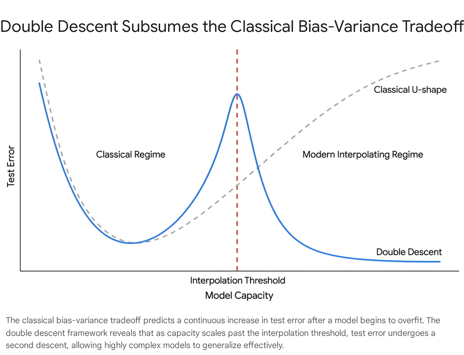
Traditional models operate under the assumption that as a model's complexity increases - whether by adding polynomial degrees, decision nodes, or features - its bias strictly decreases while its variance strictly increases 2. This dynamic produces a classical U-shaped risk curve. Test error initially decreases as the model gains the capacity to learn the underlying structure of the training data, but it eventually begins to rise rapidly as the model becomes overly flexible 367. In this high-variance regime, the model memorizes random noise and idiosyncratic training variations, leading to classical overfitting 34. Consequently, practitioners have historically relied on capacity control mechanisms, such as explicit regularization, cross-validation, and early stopping, to constrain models to an optimal intermediate complexity 348.
The Interpolation Paradox and Historical Precedents
The empirical success of modern deep learning has systematically challenged the ubiquity of the U-shaped risk curve. Contemporary state-of-the-art architectures, including highly parameterized convolutional neural networks, vision transformers, and large language models (LLMs), are routinely trained in overparameterized regimes where the number of model parameters vastly exceeds the number of training samples 78. These models are frequently optimized to achieve perfect interpolation - zero error on the training dataset - which classical theory predicts should lead to catastrophic overfitting and an explosion in test error 389. Instead, these networks demonstrate remarkable out-of-sample generalization 810.
To reconcile this contradiction, Belkin et al. (2019) popularized the concept of "double descent" 38910111213. Double descent is a phenomenon wherein a model's test error exhibits a non-monotonic trajectory as complexity scales. The error initially follows the classical U-shaped curve, dropping and then spiking to a severe peak. This peak occurs exactly at the "interpolation threshold," the critical point where the model's capacity is just sufficient to perfectly memorize the training data 3689. However, as model complexity scales beyond this threshold into the overparameterized regime, a "second descent" occurs. The test error drops again, often achieving performance superior to the optimal point of the classical underparameterized regime 691213.
While the term "double descent" was coined to address modern deep learning, the mathematical anomaly it describes has historical precedents in physics and minimum norm linear regression. Early observations date back to 1989, when Vallet et al. demonstrated a twofold descent in the learning curves of classifiers trained via pseudo-inverse solutions 91114. Similarly, Opper (1995) provided theoretical results on the phenomenon using statistical physics frameworks, and Duin (1995) documented analogous risk curves on real-world data employing pseudo-Fisher linear discriminants 11. More recently, the phenomenon has been mathematically documented as the "$m=n$ machine learning anomaly" 9. Today, double descent is recognized as a pervasive structural property across an array of architectures, manifesting in linear regression, random forests, fully connected networks, residual networks, and massive transformer models 36121516.
Typology of the Descent Phenomenon
Following its formalization, empirical research by Nakkiran et al. (2021) and others demonstrated that double descent is not isolated to static parameter counts. The phenomenon emerges across multiple axes of complexity, manifesting in model-wise, epoch-wise, and sample-wise dimensions 91214.
Model-Wise Scaling
Model-wise double descent is the most commonly analyzed variant, occurring when test error is evaluated as a direct function of architectural size 121415. In this framework, complexity scales as the model is broadened by adding wider layers, deeper network structures, or an increased volume of decision trees 14. As parameters are added, the model sequentially transitions from an underfitting regime to the critical interpolation threshold. At this exact threshold, where the number of parameters roughly matches the number of training examples ($N \approx D$), the model barely possesses the capacity to fit the dataset, resulting in a severe spike in test error 912. Continuously increasing the parameter count pushes the model into the overparameterized regime. In this space, the excess capacity allows the optimization algorithm to find smoother, more stable interpolating functions, triggering the second descent 21415.
Epoch-Wise Training Dynamics
Double descent also unfolds dynamically over training time, known as epoch-wise or time-wise double descent 1415162021. When a heavily overparameterized model undergoes gradient descent, test error typically drops initially as the model learns the broadest, most robust features of the dataset 141617. Eventually, the model exhausts these general patterns and begins to memorize the specific noise and mislabeled examples of the training set, causing the test error to rise 1417.
Classical optimization protocols rely on "early stopping" to halt training at this exact inflection point 416. However, researchers have observed that if training is allowed to continue far past the overfitting spike - often utilizing techniques like learning rate decay or weight averaging - the test error frequently falls again 142017. This occurs because extended training provides the optimizer the time necessary to traverse the loss landscape, escaping sharp minima caused by memorization and settling into flatter, more generalizable minima 41421.
Sample-Wise Data Dynamics
The most counterintuitive manifestation is sample-wise double descent, which examines test error as a function of training dataset volume 814. Fundamental machine learning principles suggest that adding more data invariably improves generalization. However, sample-wise double descent reveals a critical hazard: if a model's size is held fixed, injecting additional training data can inadvertently push the model out of a safe, overparameterized regime directly into the interpolation threshold 11415.
When the volume of data approaches the model's fixed parameter capacity, the network struggles to accommodate the new information, its noise sensitivity amplifies, and test error spikes 11415. In these specific scenarios, providing the model with more data actually degrades its performance. Generalization only recovers if the dataset is expanded massively enough to push the model firmly back into the underparameterized regime, or if the model's architecture is scaled up concurrently to maintain overparameterization 1415.
| Dimension of Descent | Definition of the "Complexity" Axis | Trigger for the Interpolation Peak | Implications for Applied Machine Learning |
|---|---|---|---|
| Model-Wise | Count of parameters, width, depth, or hidden units. | Parameter count directly equals the number of training examples ($N \approx D$). | A spike in error during model scaling does not mean scaling should stop; further scaling often recovers performance. |
| Epoch-Wise | Optimization steps, training time, or number of epochs. | The model shifts from learning generalizable features to memorizing dataset noise. | Early stopping may prematurely halt learning; extended training can unlock flatter, superior minima. |
| Sample-Wise | Total volume of training data points provided to the model. | Data volume grows to perfectly match the fixed parameter capacity of the model. | Adding incremental data can temporarily ruin performance unless model capacity is scaled simultaneously. |
Geometric and Mathematical Foundations
To explain the precise mechanics of the interpolation peak and the subsequent recovery, statistical theorists have mapped the phenomenon using the geometry of high-dimensional optimization, linear regression, and spectral analysis.
Hessian Conditioning and Noise Sensitivity
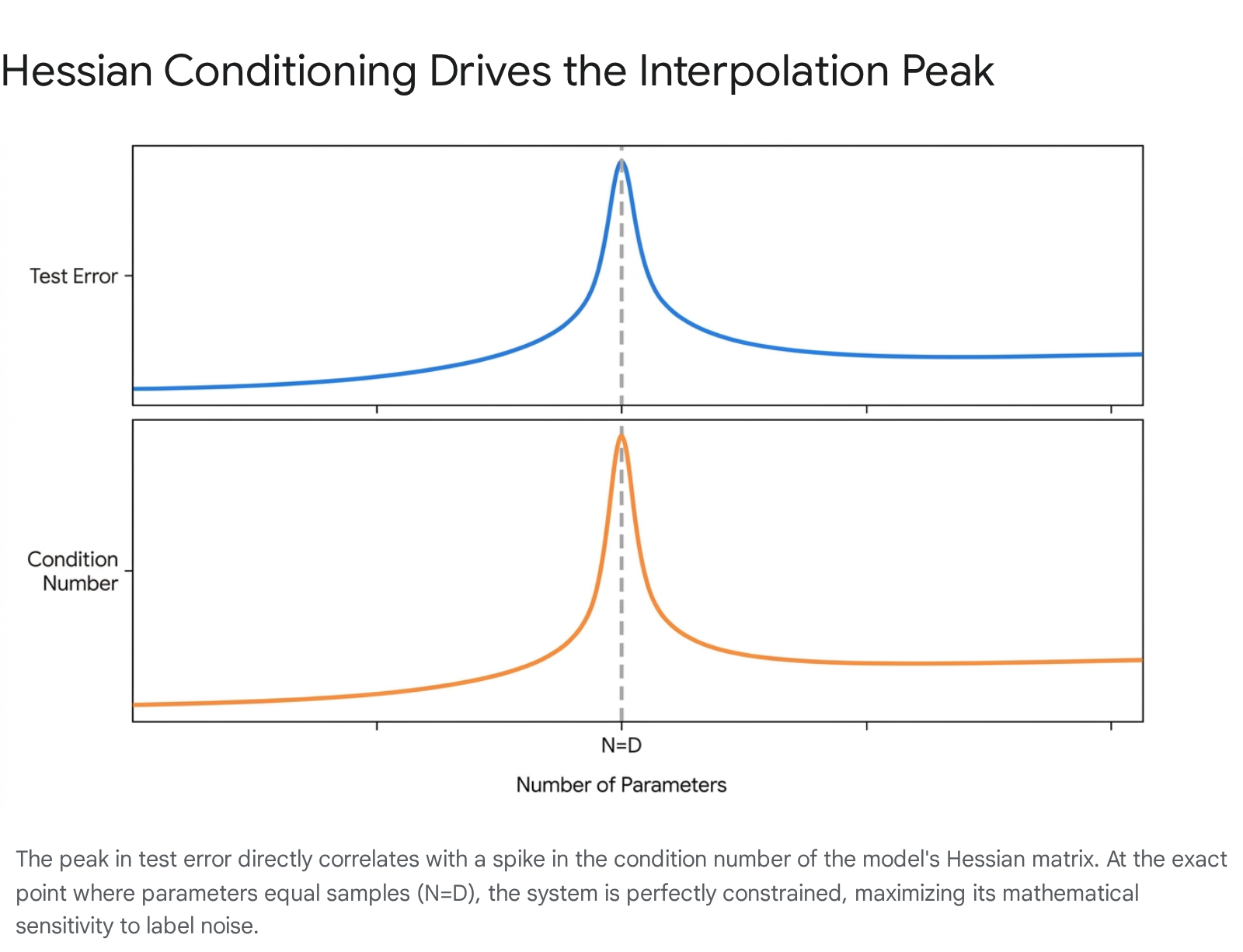
The severity of the error spike at the interpolation threshold is fundamentally driven by the mathematical condition number of the system 181925. In optimization, the condition number of the Hessian matrix (or the input data matrix) dictates how acutely the system's output will vary in response to minor perturbations or noise in the input data 19252620.
When solving a regression or classification problem where the number of parameters $D$ exactly equals the number of equations or data points $N$, the data matrix is perfectly square. In this exact configuration, assuming full rank, the matrix inverse exists and is unique 192122. However, random data matrices at $N=D$ exhibit their highest (worst) possible condition number 1922.
Because the model has zero degrees of freedom remaining, it is mathematically forced to contort its decision boundary to pass exactly through every single data point, including corrupted inputs and label noise 121. This creates a highly jagged, erratic function that wildly mispredicts unseen data 21.
Once the model transitions into the underdetermined, overparameterized regime ($D > N$), the condition number plummets 1922. In this regime, an exact matrix inverse no longer exists, but infinitely many solutions can perfectly fit the training data. This abundance of degrees of freedom allows the optimization algorithm to utilize a generalized pseudo-inverse, which reliably selects the solution with the minimum norm 111921. This minimum-norm solution is characterized by smooth mathematical behavior, effectively ignoring high-frequency noise and facilitating the second descent in test error 221.
The Amplification Role of Label Noise
Empirical analyses consistently confirm that the severity of the interpolation peak is inexorably linked to the signal-to-noise ratio within the training dataset 114151520. When models are trained on completely clean, noise-free data, double descent is frequently mitigated, manifesting as a gentle, smooth plateau rather than a destructive peak 1420.
However, introducing label noise - even purposefully mislabeling a small fraction (e.g., 10% to 20%) of the data - triggers aggressive model-wise and epoch-wise double descent 1420. As the label noise ratio increases, the test error peak rises proportionally, and the model requires a vastly larger injection of parameters to successfully exit the noisy regime and recover performance 1420. The excess capacity in the overparameterized regime serves as a geometric buffer; the model isolates the corrupted noise information into separate, non-disruptive internal representations, leaving the core predictive signal intact 14.
The Unimodal Variance Curve
To align these geometric realities with classical statistics, researchers have revisited the fundamental bias-variance decomposition. Through rigorous measurement of neural networks, Yang et al. demonstrated that the classical assertion regarding bias remains entirely accurate: as network width increases, the bias term decreases strictly monotonically 5.
The classical error occurs in the assumptions regarding variance. In deep learning models, variance does not explode to infinity in the overparameterized space. Instead, the variance curve is inherently unimodal or bell-shaped 5. Variance increases sharply as the model approaches the interpolation threshold, driving the test error spike. However, once the model crosses into the overparameterized regime, the variance begins to decrease monotonically 25. This reduction occurs because extreme parameter redundancy induces a stabilizing averaging effect across the network's components, and implicit regularization biases the optimizer toward smoother solutions 25.
Theoretical Frameworks in the Overparameterized Regime
Understanding why stochastic gradient descent (SGD) reliably finds these benign, minimum-norm solutions among infinitely many bad options has spawned several competing mathematical frameworks.
Neural Tangent Kernels (NTK) and Lazy Training
To formalize the dynamics of immense parameterization, theorists introduced the Neural Tangent Kernel (NTK) 72324. The NTK framework proves that in the limit of infinite width, the training dynamics of a fully connected neural network optimized by gradient descent become mathematically equivalent to kernel ridge regression using a deterministic, fixed kernel 72324.
In this "kernel regime," the parameters of the wide neural network change only negligibly from their random initialization during training 23. Because the kernel remains fixed, the optimization path is smooth and tightly controlled, explaining how massive capacity models avoid fitting noisy, complex patterns 24. However, the assumption that parameters barely move defines a "lazy" training regime 2325. While mathematically elegant for proving generalization bounds, the strict NTK limit precludes "active feature learning" - the ability of a network to actively shift its representations to learn hierarchical concepts, which is widely considered the true source of deep learning's empirical power 232526.
Benign Overfitting and Active Feature Learning
Closely related to double descent is the concept of "benign overfitting," popularized by Bartlett et al. (2020) 133435. Benign overfitting describes scenarios where models perfectly interpolate noisy training data yet still generalize optimally to unseen data 133527.
In theoretical models, benign overfitting requires that the data distribution possesses a specific spectral decay. The dominant eigenmodes (the core signals) are learned efficiently, while the infinite tail of low-variance eigenmodes acts as a high-dimensional buffer that absorbs the noise without meaningfully distorting the primary predictive function 2728. While initially proven only in asymptotic or infinitely high-dimensional linear settings, recent studies indicate that "almost benign overfitting" occurs in fixed dimensions for nonlinear neural networks undergoing active feature learning 25352729. In the "rich" feature-learning regime, networks actively sacrifice some margin radius to compress the intrinsic dimensionality of the data, achieving benign interpolation without relying on the fixed-kernel constraints of the NTK 2527.
Spectral-Transport Stability Theory
Seeking a unified explanation for why some models exhibit severe interpolation peaks while others interpolate benignly, researchers proposed the Fredriksson theory of spectral-transport stability 2830. This framework posits that double descent is not an inevitable consequence of parameter counting, but rather the result of a three-way interaction: 1. Spectral Geometry: The eigenvalue distribution of the training data. 2. Transport Stability: The sensitivity of the chosen optimization algorithm (the learning rule) when a single training sample is replaced. 3. Noise Alignment: How maliciously the label noise aligns with the population's core eigenmodes 2830.
Under this framework, the interpolation peak can be entirely flattened or eradicated if the effective dimension of the data grows too slowly, if the algorithm is exceptionally stable under sample replacement, or if the noise is heavily concentrated away from the primary data features 2830.
Intersections with Modern Deep Learning Dynamics
The mechanics of double descent contextualize several heavily researched phenomena in contemporary artificial intelligence, notably grokking, scaling laws, and the behavior of foundation models.
Grokking and Phase Transitions
"Grokking" is a training dynamic observed predominantly in algorithmic datasets (such as modular arithmetic), wherein a model rapidly achieves perfect training accuracy while test accuracy languishes at random chance 173132. If training is sustained for thousands of additional epochs, the model undergoes a sudden, dramatic phase transition, perfectly generalizing to the test set 3132.
Initially, grokking was treated as a distinct anomaly, separate from double descent due to its delayed onset and abruptness 173132. However, emerging consensus unifies grokking and epoch-wise double descent under a framework of competing pattern learning speeds 1732. Early in training, the network rapidly constructs a "dense" subnetwork of heuristic features that memorize the data (causing the interpolation peak) 1732. Over prolonged optimization, weight decay and gradient flow implicitly favor simpler, "sparse" subnetworks that capture the true underlying logic 232. In highly structured algorithmic tasks, this transition is a sharp phase shift (grokking); in continuous, noisy tasks like image classification, the transition is smoother and registers as the U-shaped recovery of epoch-wise double descent 41732.
Neural Scaling Laws and Data Constraints
The development of frontier LLMs relies heavily on empirical neural scaling laws, which assert that model performance (cross-entropy loss) improves as a predictable, smooth power-law function of compute, model size, and dataset size 3334443536. The highly cited Chinchilla scaling law posits that the optimal ratio for training compute dictates a linear relationship where dataset size ($D$) should roughly equal 20 times the parameter count ($N$) 364748.
Notably, standard Chinchilla power laws do not depict the double descent peak 3537. This absence is because dominant scaling laws were calibrated exclusively for the data-rich, single-epoch pretraining regime 3537. The Chinchilla formulation assumes every token processed is entirely unique, operating firmly in the underparameterized regime where model capacity is strictly the bottleneck 3537.
Data Repetition and Catastrophic Inheritance
As the global supply of high-quality internet text reaches exhaustion, frontier AI laboratories are increasingly forced to train models for multiple epochs over the same data 3537. Repeating data violently breaks the assumptions of single-epoch scaling laws and reintroduces double descent dynamics 35385139.
Research from Anthropic reveals that when even a fractional percentage of a dataset is repeated heavily during LLM training, a severe mid-training double descent peak emerges 38. The model diverts massive amounts of capacity to explicitly memorize the repeated sequences, damaging the internal induction heads responsible for broader generalization 38. In one experiment, repeating just 0.1% of the data 100 times degraded the performance of an 800-million parameter model to match that of a model half its size 38. To accurately forecast performance in data-constrained regimes, researchers are now modifying scaling laws to include additive overfitting penalties that account for the degradation caused by epoch-wise memorization 3551.
| Framework | Core Premise | Relationship to Interpolation and Generalization |
|---|---|---|
| Neural Scaling Laws (Chinchilla) | Loss falls smoothly as a power-law when $N$ and $D$ scale optimally (e.g., $D=20N$). | Bypasses double descent entirely by assuming unique data and operating strictly in the underparameterized, early-training regime. |
| Grokking | Sudden generalization occurs thousands of epochs after the model overfits the training set. | An extreme, delayed manifestation of epoch-wise double descent, transitioning sharply from a memorization circuit to a generalization circuit. |
| Data Repetition Penalties | Scaling laws break down when training tokens are not unique, causing severe performance degradation. | Reintroduces the epoch-wise double descent peak into LLM training; capacity is wasted memorizing duplicates. |
Implications for Optimization and Deployment
The validation of double descent permanently alters how machine learning engineers approach architecture design, optimization hyperparameters, and data curation.
Model Sizing and Overtraining
The discovery that excess capacity serves as an active buffer against noise invalidates the traditional heuristic that shrinking a failing model will prevent overfitting 2614. If test error spikes during scaling, the mathematically sound intervention is often to dramatically increase the parameter count until the model breaches the second descent 614.
Furthermore, while Chinchilla defines "compute optimality" for the training phase, production realities prioritize inference cost 3648. Consequently, frontier models like Meta's Llama 3 are purposefully "overtrained" far past the Chinchilla optimal point. For instance, Llama 3's 8B parameter model was trained on 15 trillion tokens - two orders of magnitude beyond the theoretical 200 billion token optimum 4853. This massive overparameterization of data to parameters yields highly capable, compressed models that are significantly cheaper to run at inference time, heavily leveraging the generalization stability found in deep descent regimes 3648. Interestingly, specialized tasks can still exhibit classical behavior; recent research on pre-training scaling laws specifically for reasoning tasks suggests that excessive scaling without architectural changes can trigger "inverse scaling," leading to a degraded, U-shaped performance curve in logic execution 54.
Hyperparameter Dependencies
Double descent is not an absolute physical law; its presence is highly dependent on the optimization landscape 2540. Research by Yilmaz and Heckel demonstrates that model-wise double descent is only observed if the optimizer successfully navigates to a sufficiently low-loss minimum 2541. Optimization choices directly influence the condition number of the descent path. If a model is trained with an inappropriately low learning rate or an excessively large batch size, it will fail to reach the interpolation threshold effectively, resulting in an aborted training run where the double descent peak is diminished or absent 25.
Data Management and Regularization
Sample-wise double descent acts as a rigorous warning against indiscriminate data collection 114. When a model approaches the interpolation threshold, dumping uncurated, noisy data into the training pipeline will actively amplify noise sensitivity and trigger a generalization collapse 1. Practitioners must rely on active learning, deduplication, and stratified sampling to safely cross the threshold 139.
Additionally, while overparameterized gradient descent provides implicit regularization, explicit techniques like weight decay (L2 regularization) remain critical. Adequate regularization suppresses the condition number of the Hessian by enforcing smaller parameter norms, effectively smoothing the erratic functional fits at the interpolation peak and mitigating the severity of the double descent spike 415.